Lagrangian Optimization of Wall Injected Flows

I am pleased to share some of the results of my research over the past few years. These just appeared as a review article in the Proceedings of the Royal Society A and you can download it from here (and the cool thing about the Royal Society – besides its very professional reviewers – review articles are free access to everyone!)

http://dx.doi.org/10.1098/rspa.2009.0326

I hope that you will enjoy reading this manuscript as it includes many classical ideas with a novel twist as well as some original derivations and solutions for flows at large Reynolds numbers.

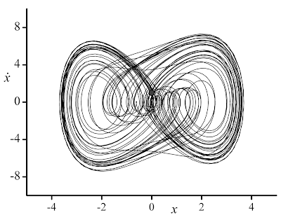
The heart of this research resides in the fact that we were able to capture solutions that range from purely irrotational to highly rotational fields using a single formulation. These have different energy signatures and morph according to the energy level they are at. The second law of thermodynamics is then used to identify which of those solutions is the most likely to occur in practice based on the entropy maximization principle. Finally, Kelvin’s minimum energy theorem is extended to open regions thus granting it applicability to a wider class of problems. It is used here to prove that the solution with minimum kinetic energy corresponds indeed to the irrotational motion.

Working on this article is one of the main reasons that I have not been posting recently,

Cheers!

Cite as:
Saad, T. "Lagrangian Optimization of Wall Injected Flows". Weblog entry from Please Make A Note. http://pleasemakeanote.blogspot.com/2009/10/lagrangian-optimization-of-wall.html

How to add space after \hline in LaTeX tables

Try the following:

\hline \\[-1.0em]

Voila!

Of course, you can change the numbers and units inside the brackets.

Cite as:
Saad, T. "How to add space after \hline in LaTeX tables". Weblog entry from Please Make A Note. http://pleasemakeanote.blogspot.com/2009/08/how-to-add-space-after-hline-in-latex.html

How to highlight text in LaTeX

Add the following to your preamble:

\usepackage{color}
\newcommand{\hilight}[1]{\colorbox{yellow}{#1}}

To highlight text in the body of your document, use

\hilight{this is some highlighted text}

Voila!

Of course, you can change the color from yellow to any of the supported colors. For a list of those, check: http://en.wikibooks.org/wiki/LaTeX/Colors

UPDATE:

There is a problem with the previous method is that the color box does not wrap properly. Here's a much easier and robust way of doing this

\usepackage{soul}

To highlight text in the body of your document, use

\hl{this is some highlighted text}

Cite as:
Saad, T. "How to highlight text in LaTeX". Weblog entry from Please Make A Note. http://pleasemakeanote.blogspot.com/2009/08/how-to-highlight-text-in-latex.html

OriginLab Settings for High Quality Graphs

This is a well overdue post. I know that some readers have been waiting for this. I apologize for the delay. I hope you'll find this talk useful.

Cite as:
Saad, T. "OriginLab Settings for High Quality Graphs". Weblog entry from Please Make A Note. http://pleasemakeanote.blogspot.com/2009/06/originlab-settings-for-high-quality.html

Flashget Script Error/Flashget Recommends bar

In Flashget, go to:

View/Recommendation

and uncheck it.

Obviously, the ads displayed by flashget are generating an internet explorer script error. I never liked that recommend bar anyway.

Cite as:
Saad, T. "Flashget Script Error/Flashget Recommends bar". Weblog entry from Please Make A Note. http://pleasemakeanote.blogspot.com/2009/06/flashget-script-errorflashget.html

hyperref and pdfdraftcopy

There seems to be a problem when these two packages are used together. Try adding the following to your preamble – it worked well on my end

\makeatletter
    \def\@DRAFTdimen{% copied from pdfdraftcopy.sty 
    \setlength\LLY{\paperheight} 
    \addtolength\LLY{-\textheight} 
    \addtolength\LLY{-\headheight} 
    \addtolength\LLY{-\headsep} 
    \addtolength\LLY{-1in} 
    \addtolength\LLY{-3pt} 
    \setlength\LLX{1in} 
    \ifodd\value{page}% was \thepage 
    \addtolength\LLX{\oddsidemargin}\else 
    \addtolength\LLX{\evensidemargin}\fi 
    \setlength\URX{\textwidth} 
    \setlength\URY{\textheight}
}
\makeatother

Voila!

Cite as:
Saad, T. "hyperref and pdfdraftcopy". Weblog entry from Please Make A Note. http://pleasemakeanote.blogspot.com/2009/06/hyperref-and-pdfdraftcopy.html

Make Nomenclature in WinEdt

First, you need to download this file

http://www.winedt.org/Macros/LaTeX/MakeNomencl.php

Save it in the “Exec/MiKTeX” folder under your WinEdt path, e.g.

C:\Program Files\Winedt Team\WinEdt\Exec\MiKTeX

in WinEdt, do the following

1. Right click on the Menu bar
2. Select “Menu Steup”
3. Double click on any of the menus where you would like your make nomenclature command to go (Accessories would be a good candidate)
4. On your upper left, choose Insert->Macro
5. Name the new command (Make Nomenclature)
6. Under Macro, type the following: Exe('%b\Exec\MiKTeX\MakeNomencl.edt');

Voila!

Cite as:
Saad, T. "Make Nomenclature in WinEdt". Weblog entry from Please Make A Note. http://pleasemakeanote.blogspot.com/2009/06/make-nomenclature-in-winedt.html

7zip Batch Zip

First, make sure that the 7zip directory is in your path. Usually, it is located at

C:\Program Files\7-Zip

Next, write the following in batch file

Zip all files in a directory

for /f %%A in ('dir /b') do 7z a -tbzip2 "%%A.bz2" "%%A"

Zip files with a specific extension in a directory (download batch file)

for /f %%A in ('dir /b *.txt *.dat') do 7z a -tbzip2 "%%A.bz2" "%%A"

Save and run in the directory where you want to zip the files.

Here, I am compressing using bzip2 (notice the switch: –tbzip2). You can change that to

-tzip for zip

-tgz for gz

-t7z for 7z

some more examples here.

Cite as:
Saad, T. "7zip Batch Zip". Weblog entry from Please Make A Note. http://pleasemakeanote.blogspot.com/2009/05/7zip-batch-zip.html

Restart Windows in Remote Desktop

press:

Alt + F4

Voila!

Cite as:
Saad, T. "Restart Windows in Remote Desktop". Weblog entry from Please Make A Note. http://pleasemakeanote.blogspot.com/2009/05/restart-windows-in-remote-desktop.html

How to Add a Watermark in Latex

More often than not, I like to place a “DRAFT” watermark on my documents. This can be easily and automatically done by just including a specific package (one for PS and one for PDF).

Here’s how

\usepackage[draftcopy] % for PS and DVI

\usepackage[pdfdraftcopy] % for PDF

Voila!

For the documentation of draftcopy check here.

For the documentation of pdfdraftcopy check here.

Cite as:
Saad, T. "How to Add a Watermark in Latex". Weblog entry from Please Make A Note. http://pleasemakeanote.blogspot.com/2009/05/how-to-add-watermark-in-latex.html

Wolfram Alpha

It has been finally released!

http://www.wolframalpha.com/

I’m too sleepy now to experiment with it.

In the meantime, you can check the walking randomly blog.

Cite as:
Saad, T. "Wolfram Alpha". Weblog entry from Please Make A Note. http://pleasemakeanote.blogspot.com/2009/05/wolfram-alpha_19.html

How to Cite a Blog & Automatically Generate Citations for your Blog

The MLA format for citing a blog is:

Last Name, First. "Title of Entry." Weblog Entry. Title of Weblog. Date Posted. Date Accessed (URL).

You can find more information on studenthacks and on the Purdue website.

Now comes the fun part. If you’re familiar with the Wolfram mathworld website, there is a “CITE THIS AS” section at the bottom of every page (example). I wanted to reproduce something similar for my blog. As you may have already noticed, there is a “Cite as” box at the bottom of every post. Of course, I didn’t go over every post to add a cite-as box. I used the google blogger API to automatically add this to every post. Here’s how you can reproduce it for your own blog

1. Go to the “Edit HTML” section for your template
2. Enable the “Expand Widget Templates” check box
3. Scroll down (or search: Ctrl + f) for
   <data:post.body/>
   This may require some tweaking as your template may be different. The idea is to locate the “post body” section – right after the body text of your post.
   
4. Copy the following HTML code:
   

   <!-- BEGIN CITE AS CODE - BY T. SAAD -http://pleasemakeanote.blogspot.com --> 
   <br/> 
   <p style='border-width:1px;border-style:solid;border-color:orange; padding:4px'> 
   <font color='orange'> 
   Cite as: 
   <br/> 
   LAST NAME, FIRST NAME &quot;<data:post.title/>. 
   &quot; Weblog entry from <a href='http://LINK-TO-YOUR-BLOG> <data:blog.title/></a>. 
   <a expr:href='data:post.url'><data:post.url/></a> 
   </font> 
   </p>
   <br/> 
   <!-- END CITE AS CODE –> 



5. Save your template

Voila! Don’t forget to put your name and the link to your blog. You can easily modify the above script with little HTML and CSS knowledge.

Cite as:
Saad, T. "How to Cite a Blog & Automatically Generate Citations for your Blog". Weblog entry from Please Make A Note. http://pleasemakeanote.blogspot.com/2009/05/how-to-cite-blog-automatically-generate.html

Modifying Mathematica Menus

UPDATE - FRIDAY MAY 15, 2009
The same procedure applies for Mathematica 7.x - just look in the 7.0 directory. For convenience, I posted the Mathematica 7.0.1 modified menu file. Of course, there is no guarantee that this will work on your end, so by all means do backup your copy of the MenuSteup.tr file before using this one. You can download it from here.

UPDATE - MONDAY JUNE 02, 2008
As was kindly pointed out by an anonymous comment, Mathematica version 6.0.2 includes the "Evaluate Notebook" menu item. Also, removing the backup files from the MenuSetup directory is a must. - Thanks

In Mathematica 6.x, a couple of nice features are missing, namely, the "Evaluate Notebook" menu command and the placement of the "Quit Kernel" command. First, the "Evaluate Notebook" is completely missing form the "Evaluation" menu - and I don't see the reason for removing such a useful command from the new version. Regarding the "Quit Kernel", which is probably the most used command during a Mathematica session, is now located under Evaluation/Quit Kernel/Local. Instead of keeping that command one level higher (i.e. Evaluation/Quit Kernel), for some reason it was placed under a sub-menu.

Yesterday, I found out that one can modify the whole Mathematica menu, and in the process, add the "Evaluate Notebook" command and modify the location of the "Quit Kernel" command. Thanks to the Walking Randomly blog for sharing this information - you can find the original post here.

So here's what I have done on my end to make my Mathematica workspace fit to my needs.

1. Locate the file "MenuSetup.tr" - This is usually found somewhere within the "Wolfram Research" directory. A simple search would be enough to find that file. (try C:\Program Files\Wolfram Research\Mathematica\6.0\SystemFiles\FrontEnd\TextResources\Windows\)
   
2. Open "MenuSetup.str" with a text editor. In windows, I use wordpad to do that because it keeps the formatting correct and wraps the text quite nicely.
3. Scroll down to the end of the file and locate the last brace-then-bracket "}]" then add the following before that
1. Type a comma then go to a new line
   
2. Insert the following
   Delimiter,
   Item["Evaluate &Notebook", "EvaluateNotebook"],
   
   Item["&Quit Local Kernel", "MenuListQuitEvaluators", MenuAnchor->True]
   

Voila!

You should be able to see two new menu items on the menu bar. Make sure also to backup your original MenuSetup.tr. If nothing shows up on the Mathematica menu, you might have to move the backup copy from the MenuSetup directory.

Cite as:
Saad, T. "Modifying Mathematica Menus". Weblog entry from Please Make A Note. http://pleasemakeanote.blogspot.com/2008/05/changing-mathematica-menus.html

Calling Gnuplot from c Using Pipes... Again!

Here's another way of calling gnuplot. I like this method because it provides a standalone function that plots your results. Here's the code:

#include <stdio.h>
#include <stdlib.h>
#include <math.h>
void plotResults(double* xData, double* yData, int dataSize);
int main() {
  int i = 0;
  int nIntervals = 100;
  double intervalSize = 1.0;
  double stepSize = intervalSize/nIntervals;
  double* xData = (double*) malloc((nIntervals+1)*sizeof(double));
  double* yData = (double*) malloc((nIntervals+1)*sizeof(double));
  xData[0] = 0.0;
  double x0 = 0.0;
  for (i = 0; i < nIntervals; i++) {
      x0 = xData[i];
      xData[i+1] = x0 + stepSize;
  }
  for (i = 0; i <= nIntervals; i++) {
      x0 = xData[i];
      yData[i] = sin(x0)*cos(10*x0);
  }
  plotResults(xData,yData,nIntervals);
  return 0;
}
void plotResults(double* xData, double* yData, int dataSize) {
  FILE *gnuplotPipe,*tempDataFile;
  char *tempDataFileName;
  double x,y;
  int i;
  tempDataFileName = "tempData";
  gnuplotPipe = popen("c:\\gnuplot\\bin\\pgnuplot -persist","w");
  if (gnuplotPipe) {
      fprintf(gnuplotPipe,"plot \"%s\" with lines\n",tempDataFileName);
      fflush(gnuplotPipe);
      tempDataFile = fopen(tempDataFileName,"w");
      for (i=0; i <= dataSize; i++) {
          x = xData[i];
          y = yData[i];            
          fprintf(tempDataFile,"%lf %lf\n",x,y);        
      }        
      fclose(tempDataFile);        
      printf("press enter to continue...");        
      getchar();        
      remove(tempDataFileName);        
      fprintf(gnuplotPipe,"exit \n");    
  } else {        
      printf("gnuplot not found...");    
  }
} 

This code should run as is. Of course, feel free to take the plot function and use it in your own codes.

Cite as:
Saad, T. "Calling Gnuplot from c Using Pipes... Again!". Weblog entry from Please Make A Note. http://pleasemakeanote.blogspot.com/2009/05/calling-gnuplot-from-c-using-pipes.html

Wolfram Alpha

I can't wait for this to be released!

http://www.wolframalpha.com/index.html

In the meantime, check out this presentation by Stephen Wolfram himself



or this CNET demonstration

Cite as:
Saad, T. "Wolfram Alpha". Weblog entry from Please Make A Note. http://pleasemakeanote.blogspot.com/2009/05/wolfram-alpha.html

How to Call Gnuplot from c Using Pipes (Windows)

Try this:

// Open a pipe to gnuplot
FILE *gnuplotPipe = popen("c:\\gnuplot\\bin\\pgnuplot -persist","w");
// If gnuplot is found
if (gnuplotPipe) {
  // using fprintf on the gnuplotPipe, we can directly issue commands in gnuplot
  fprintf(gnuplotPipe, "set style data lines\n");
  fprintf(gnuplotPipe, "cd 'C:\\gnuplot\\bin'\n");
  // assuming your data file is placed in the gnuplot bin directory
  fprintf(gnuplotPipe, "plot \"data-file.dat\" using 1:2\n");
  fflush(gnuplotPipe);
  fprintf(stderr,"Press enter to continue...");
  fflush(stderr);
  getchar();
  // exit gnuplot
  fprintf(gnuplotPipe,"exit \n");
  pclose(gnuplotPipe);
}

Cite as:
Saad, T. "How to Call Gnuplot from c Using Pipes (Windows)". Weblog entry from Please Make A Note. http://pleasemakeanote.blogspot.com/2009/05/how-to-call-gnuplot-from-c-using-pipes.html

One year anniversary – Please Make a Note

Today marks the one year anniversary of Please Make a Note! This idea that started as a mere way of keeping track of how I accomplished certain tasks so that I can refer to them later has had an unexpected (positive) outcome: the number of visitors to this blog. Although I had wished (as everybody who owns a blog does) to reach as many online users as possible, I had never expected the current results. I am also quite pleased with the several hits that PMAN received from some important bloggers and software companies (yes!!! PMAN was visited by Mathematica people!).

In any event, I would like to thank all those who have shown interest in this blog. I hope that you found some useful posts here.

This is the monthly visits report from statcounter (12 May 2008 – 12 May 2009).

(P.S. I have no idea what happened in march!)

	Page Loads	Unique Visitors	First Time Visitors	Returning Visitors
Total	41,947	27,326	23,797	3,529
Average/month	3,227	2,102	1,831	271

Voila!

Cite as:
Saad, T. "One year anniversary – Please Make a Note". Weblog entry from Please Make A Note. http://pleasemakeanote.blogspot.com/2009/05/one-year-anniversary-please-make-note.html

How to Flatten or Embed Comments in a PDF using Acrobat©

Most often than not, I implement all my comments to PDF files (such as manuscript proofs) using the many rich features of Adobe’s Acrobat Professional. However, I always prefer to “flatten” these comments that is, make them a permanent part of the PDF document. There are a few methods for doing this, but by far, the fastest and most clever is this one, found on PlanetPDF

1. In Acrobat professional, type “Ctrl + j” to invoke the java script dialog
2. In that dialog, type: this.flattenPages();
3. press “Ctrl + Enter”

Voila!

Don’t forget to save your document.

Cite as:
Saad, T. "How to Flatten or Embed Comments in a PDF using Acrobat©". Weblog entry from Please Make A Note. http://pleasemakeanote.blogspot.com/2009/05/how-to-flatten-or-embed-comments-in-pdf.html

EndNote to JabRef to EndNote

1. In Endnote, select the citations you want to export and go to “File / Export”
2. Select “RefMan (RIS) Export” in the Output Styles dropdown box
   (in case it is not there, choose “Select Another Style…” and look for RefMan RIS Export)
3. After exporting the file, go to JabRef and import as RIS

 

Voila!

There are many ways of doing this. Here’s one on fellow blog Fundamental Thinking. Josh’s method is based on the JabRef Endnote Export Filter.

To go from JabRef to Endnote

1. In JabRef, select the citations you want to export and go to “File / Export”
2. Select “Endnote” from the dropdown box
3. In Endnote go to “File / Import”
4. Choose the data file that you just exported from JabRef
5. Under import option, choose “EndNote Import”

Voila!

Cite as:
Saad, T. "EndNote to JabRef to EndNote". Weblog entry from Please Make A Note. http://pleasemakeanote.blogspot.com/2009/04/endnote-to-jabref-to-endnote.html

How to Resolve or Link to a DOI

Given a DOI number (for a journal manuscript for instance) one can link to this DOI in a word document for example or in an HTML page by invoking the following

http://dx.doi.org/YOUR-DOI-NMBER

Try this for example

http://dx.doi.org/10.1103/PhysRev.47.777

Voila!

The DOI, or Digital Object Identifier system, is a systematic way of identifying digital resources in a rather permanent way. It is a neat way for tracking and managing digital resources in an absolute reference manner. So, for example, if you want to link to a journal paper, you can either use the permalink for that specific paper or simply link to the DOI. In theory, no matter what happens, the DOI number will always locate that paper.

Cite as:
Saad, T. "How to Resolve or Link to a DOI". Weblog entry from Please Make A Note. http://pleasemakeanote.blogspot.com/2009/04/how-to-resolve-or-link-to-doi.html

The Story with Euler…

Recently, I have been deeply immersed in studying some of Euler’s original works (based on translations where applicable, of course). Here is my conclusion:

Whatever you think you have discovered… Euler may have beaten you to it!

and yes… please quote me for that one!

I made it a necessary condition in my research, and before publishing any manuscript, to check with Euler first. Many of his results and especially the intricate steps of his derivations are lost within the edifices of his collected works (or simply because later generations of mathematicians have superseded his proofs with modern versions). Yet, you will be surprised to find in one of those steps, the exact same thing that you may be currently discovering!

Cite as:
Saad, T. "The Story with Euler…". Weblog entry from Please Make A Note. http://pleasemakeanote.blogspot.com/2009/03/story-with-euler.html

Discussing the Divine Comedy with Dante

Check out this 2006 oil painting by Dai Dudu, Li Tiezi, and Zhang An.

Click on the image to see a larger version with an image map and wiki links for the people featured in the image. There are few inaccuracies in this version, but this version has more accurate data.

Cite as:
Saad, T. "Discussing the Divine Comedy with Dante". Weblog entry from Please Make A Note. http://pleasemakeanote.blogspot.com/2009/03/discussing-divine-comedy-with-dante.html

An Easy to Use Free IDE for C/C++

I know that you’ve always wondered about what C/C++ compiler and IDE to use under windows. While Microsoft offers its version of the C/C++ compiler, many people still prefer to use the GNU suite of compilers. This, without mentioning the fact that you will need to install visual studio or, if not, manually compile your code, which should be a prehistoric task by now because there are things called IDEs that take care of that.

The other hassle about installing the GCC (GNU C Compiler) under windows, is that you have to first install MingW.

I recently found this excellent and easy to use free IDE that does everything for you. It is called Code::Blocks. This program is very easy to use, intuitive, and installs the GCC compiler and MingW for you.

Voila!

Cite as:
Saad, T. "An Easy to Use Free IDE for C/C++". Weblog entry from Please Make A Note. http://pleasemakeanote.blogspot.com/2009/03/easy-to-use-free-ide-for-cc.html

The Illusion of Knowledge

Although not along the general theme of this blog, I am obligated to make this post so that I remember this, and hopefully, share it with many other fellow engineers and researchers.

I was deeply motivated and moved by a quote from Daniel J. Boorstin:

The greatest obstacle to discovery is not ignorance, it is the illusion of knowledge.

Indeed, often times we find ourselves locked within an bubble of knowledge, thinking that we know everything and that we have solutions for all, yet, we fail to realize that this only an imaginary crust beyond which lies the unknown.

Cite as:
Saad, T. "The Illusion of Knowledge". Weblog entry from Please Make A Note. http://pleasemakeanote.blogspot.com/2009/02/illusion-of-knowledge.html

8. Derivation of the Continuity Equation in Cylindrical Coordinates

This is one of my favorite derivations. Although it would sound a bit intimidating at first, as none of the standard textbooks carry out the derivation in curvilinear coordinates; it is rather easy to obtain. And guess what? the math is quite rewarding!
So we first have to start by selecting a convenient control volume. The idea here is to pick a volume whose sides are parallel per say to the coordinates. For cylindrical coordinates, one may choose the following control volume

Again, as we did in the previous post, we need to account for all the fluid that is accumulating, and flowing through this control volume, namely:
Rate of Rate of Flow In = Accumulation  + Rate of Flow Out
or
Accumulation + Flow Out - Flow In = 0

First, let’s get some basics laid out. The velocity field will be described as

I always prefer to use u, v, and w instead of ur, utheta, and uz to save on subscripts, although the latter nomenclature is a bit more descriptive… we’ll get used to it. Now, by construction, the volume of the differential control volume is

while the mass of fluid in the control volume is

The rate of change of mass or accumulation in the control volume is then

For the net flow through the control volume, we deal with it one face at a time. Starting with the r faces, the net inflow is

while the outflow in the r direction is

So that the net flow in the r direction is

Being O(dr^2), the last term in this equation can be dropped so that the net flow on the r faces is

The net flow in the theta direction is slightly easier to compute since the areas of the inflow and outflow faces are the same. At the outset, the net flow in the theta direction is

We now turn our attention to the z direction. The face area is that of a sector of angle d\theta:

then, the inflow at the lower z face is

while the outflow at the upper z face is

Finally, the net flow in the z direction is

Now we can put things together to obtain the continuity equation

dividing by dV and rearranging the r components of the velocity

Voila!
[Previous: Continuity Eq. in Cartesian Coordinates]

[Table of Contents]

[Next: Continuity Eq. in Spherical Coordinates]

Cite as:
Saad, T. "8. Derivation of the Continuity Equation in Cylindrical Coordinates". Weblog entry from Please Make A Note. http://pleasemakeanote.blogspot.com/2009/02/8-derivation-of-continuity-equation-in.html

7. Derivation of the Continuity Equation in Cartesian Coordinates

[Previous Article: How Euler Derived the Continuity Equation]
The continuity equation is an expression of a fundamental conservation principle, namely, that of mass conservation. It is a statement that fluid mass is conserved: all fluid particles that flow into any fluid region must flow out. To obtain this equation, we consider a cubical control volume inside a fluid. Mass conservation requires that the the net flow through the control volume is zero. In other words, all fluid that is accumulated inside the control volume (due to compressibility for example) + all fluid that is flowing into the control volume must be equal to the amount of fluid flowing out of the control volume.
Accumulation + Flow In = Flow Out

The mass of the control volume at some time t is

The time rate of change of mass in the control volume is

Now we can compute the net flow through the control volume faces. Starting with the x direction, the net flow is

Similarly, the net flow through the y faces is

while that through the z faces is

Upon adding up the resulting net flow and diving by the volume of the fluid element (i.e. dxdydz), we get the continuity equation in Cartesian coordinates

Voila!

Cite as:
Saad, T. "7. Derivation of the Continuity Equation in Cartesian Coordinates". Weblog entry from Please Make A Note. http://pleasemakeanote.blogspot.com/2009/02/derivation-of-continuity-equation-in.html

The Coming Revolutions in Theoretical Physics

Check out this interesting talk by David Gross

Cite as:
Saad, T. "The Coming Revolutions in Theoretical Physics". Weblog entry from Please Make A Note. http://pleasemakeanote.blogspot.com/2009/02/coming-revolutions-in-theoretical.html

Windows Defender Update Issues

For some reason, windows defender starts messing up and is not able to detect the latest updates. You will then need to download and install these updates manually. Check this out

How to troubleshoot definition update issues for Windows Defender

I hope that works out for you.

Cite as:
Saad, T. "Windows Defender Update Issues". Weblog entry from Please Make A Note. http://pleasemakeanote.blogspot.com/2009/02/windows-defender-update-issues.html

Enable the Vorticity Magnitude Computation in Fluent Inviscid Simulations

For inviscid models, Fluent does not allow you to compute the vorticity magnitude. While it should usually be available under the velocity section of the variables to plot, an inviscid fluent model lacks this feature. I am not sure why this is the case as inviscid flows are generally rotational! Only irrotational flows have zero vorticity.

So any way, some of my models are run under inviscid flow conditions and to compute the vorticity, one may define a UDF to compute it or simply export the velocity field data and compute it in a data analysis software. I find this rather cumbersome as it cost me a lot of time and the accuracy of my computations may suffer a bit. It could have been just easier if Fluent does that automatically.

Here’s a neat trick: to enable the computation of vorticity in an inviscid Fluent model, simply change your model to laminar and you’ll see that nice vorticity magnitude variable show up!

Go to: Define/Models/Viscous and select Laminar

Voila!

Of course, you should do this after you’re done with your inviscid simulation.

Cite as:
Saad, T. "Enable the Vorticity Magnitude Computation in Fluent Inviscid Simulations". Weblog entry from Please Make A Note. http://pleasemakeanote.blogspot.com/2009/02/enable-vorticity-magnitude-computation.html

Derivation of the Navier Stokes and Fluid Transport Equations

In this series:

1. The Material Derivative
   
   1. Cartesian Coordinates
   2. Cylindrical Coordinates
   3. Spherical Coordinates
   4. Vector Form
2. The Reynolds Transport Theorem
3. The Continuity Equation
   1. How Euler Derived the Continuity Equation
   2. Cartesian Coordinates
   3. Cylindrical Coordinates
   4. Spherical Coordinates
4. The Momentum Equations
   1. How Euler Derived the Momentum Equations
   2. Cartesian Coordinates
   3. Cylindrical Coordinates

Cite as:
Saad, T. "Derivation of the Navier Stokes and Fluid Transport Equations". Weblog entry from Please Make A Note. http://pleasemakeanote.blogspot.com/2008/08/derivation-of-navier-stokes-equations_16.html

6. How Euler Derived the Continuity Equation

[Previous Article: The Reynolds Transport Theorem]

I thought that it would be interesting to present Euler’s derivation of the continuity equation for incompressible flows. Although d’Alembert, in 1752, had already presented an equivalent equation in his Essai d’une nouvelle théorie de la résistance des fluides (which he had already submitted to the Academy of Sciences of Berlin in 1749), the one proposed by Euler in 1756 (written 1752) is considered to be the most rigorous.

Euler’s contribution to Fluid Mechanics goes beyond what a scientist may imagine, and was mostly due to four manuscripts published between 1752 and 1755. These are

1. Principia Motus Fluidorum (1756) [pdf]
2. Principes généraux de l’état d’équilibre des fluides (1755) [pdf]
3. Principes généraux du mouvement des fluides (1755) [pdf]
4. Continuation des recherches sur la théorie de mouvement des fluides (1755) [pdf]

The final thing I would like to point out is that Euler’s genius lies partly in his ability to synthesize and introduce world class notation. In this way, he was able to supersede all his predecessors.

Without further ado, let’s begin.

Euler starts by saying:

“… I shall posit that the fluid cannot be compressed into a smaller space, and its continuity cannot be interrupted. I stipulate without qualification that, in the course of the motion within the fluid, no empty space is left by the fluid, but it always maintains continuity in this motion…” [Paragraph 6, Principia Motus Fluidorum, Translated by Enlin Pan]

He then argues that if one considers any part of a fluid of this type (i.e. incompressible), then each individual particles fill the same amount of space as they move around. He then infers that if this happens for particles, it should happen to the fluid as a whole (which was his assumption of incompressibility). One is now able to consider an arbitrary fluid element and then track its instantaneous changes ”to determine the new portion of space in which it will be contained after a very small time period”. The amount of space that is occupied by the fluid element after it moves with time should then be equal in size to the old one. This is simply brilliant! Euler says that “this equating of size will fully characterize what can be said about the motion”.

To do this, Euler considers an initial fluid element whose shape is a right triangle. Below is the actual drawing from his manuscript:

Figure 1

Here’s an advanced version of his figure

Figure 2

The ABC triangle is our initial fluid element with an initial area

Euler then assigns a velocity field at the base vertex A as

Accordingly, the velocities of vertices B and C can be calculated as

and

For a differential time increment, the fluid element ABC will translate, rotate, and stretch while maintaining the same surface area. This is the key to the derivation as mentioned earlier. So the next order of business is to estimate the area of the triangle A’B’C’ and set it equal to that of ABC. if

then

subsequently, one can evaluate the position vectors of the remaining vertices

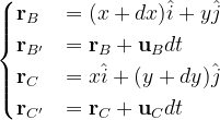
Now we have all the required equations to evaluate the area of A’B’C’. For simplicity, we’ll use the cross product. We have

Upon a pretty cool evaluation, (which I won’t illustrate here but I still think that you should carry it over because things cancel out very nicely), we obtain

Finally, here’s the punch line. By equating S’ and S, we obtain

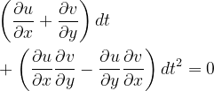
or

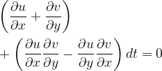
Euler then argues that the second term in this last equation is vanishingly small compared to the first term and in the limit of an infinitesimal time increment, we obtain what we call today the continuity equation

Q.E.D

I would like to thank the Euler archive for doing a great service for humanity by archiving Euler’s works as well as providing translations for some of his texts. The quoted paragraphs in orange are taken from Enlin Pan's english translation of Euler’s Principia Motus Fluidorum.

[Previous Article: The Reynolds Transport Theorem]

[Next Article: The Continuity Equation in Cartesian Coordinates]

Cite as:
Saad, T. "6. How Euler Derived the Continuity Equation". Weblog entry from Please Make A Note. http://pleasemakeanote.blogspot.com/2009/02/derivation-of-navier-stokes-equations.html

Setting Column Values in Origin – the Programmers Way!

Do the following

1. Select any of the columns by clicking on its title label
2. Right click and invoke the “Set Values” dialog box
3. Click on the little arrow to the bottom right (“Show Scripts”)
4. In the “Before Formula Scripts” text box, type in the following:
   // set your reference paramters
   aRef = 10;
   aCorrection = 0.01;
   // loop over columns – say from column 2 to column 25 – you may need to start at column 2
   // since column 1 usually holds the data corresponding to the independent variable
   loop(i, 2, 25) {
   wcol(i) /= aRef;
   wcol(i) += aCorrection;
   }
   
5. Click “Apply” or “OK”
   

Voila!

Origin is a “professional data analysis and graphing software for sicnetists and engineers”. More often than not, I find myself importing tons of data into worksheets. Most of the time, I would be comparing analytical (yes, some folks on this planet still do analytical work) and numerical data. Without loss of generality, most analytical solutions produce dimensionless data which will eventually end up being compared to numerical or experimental results. Of course, the numerical or experimental results need to be normalized accordingly. Bottom line, you have to go through every column of external data and do what needs to be done: divide, multiply, subtract etc…

In Origin, once you have some values in a column, you can right click on that column and select “Set Column Values” and enter some formula (e.g. Col(A) = Col(A)*10 + 2). The brute force approach is to go over every column, and type in the formula over and over again. So for Column B, you’ll have Col(B) = Col(B)*10 + 2 and so on.

Fortunately, Origin is amazingly modular and allows you to put in your formulas as a script. So here’s the idea: How about writing a script that loops over all the desired columns and sets the values accordingly?

The nice thing about this is that you can use the usual C operations: *=, /=, +=, and –=.

For online video tutorials and goodies related to Origin, check the OriginLab Website.

Enjoy programming!

Update: A couple of graphs made using Origin to illustrate the quality of the resulting graphs. Note that the default graph template used by Origin may look just like an excel graph. You will have to customize your graph to match the look that you are looking for, and of course, reuse the template you have created.

Cite as:
Saad, T. "Setting Column Values in Origin – the Programmers Way!". Weblog entry from Please Make A Note. http://pleasemakeanote.blogspot.com/2009/02/setting-column-values-in-origin.html

LaTeX: Vertical Spacing in Multiline Equations

To add some extra spacing in multiline equation environments (such as align or gather), you can use the \jot command either in the preamble which will affect all your multiline equations, or only locally.

\setlength{\jot}{height}

Here’s an example

\begin{align*}
\setlength{\jot}{12pt}
a + c^3 & = 0 \\
a + b^2 & = 0 \\
d + c^{-1} & = 10 \\
d + a^2 & = \pi
\end{align*}

it looks like this

Voila!

ref: LaTeX Community

Cite as:
Saad, T. "LaTeX: Vertical Spacing in Multiline Equations". Weblog entry from Please Make A Note. http://pleasemakeanote.blogspot.com/2009/02/latex-vertical-spacing-in-multiline.html

Number Theory: Mathematical Playgound

I recently received some interesting mathematical equalities

 

Just amazing!

Cite as:
Saad, T. "Number Theory: Mathematical Playgound". Weblog entry from Please Make A Note. http://pleasemakeanote.blogspot.com/2009/02/number-theory-mathematical-playgound-1.html

LaTeX: Undefined Control Sequence \printglossary

This happens when updating to the latest version of MiKTeX. Assuming that you are including the “nomencl” package, then you need to do the following substitutions:

1. Replace \makeglossary with \makenomenclature
2. Replace \printglossary with \printnomenclature

Voila!

ref: Somacon

The nomencl package is useful for producing nomenclatures/glossaries. For more information check the nomencl package documentation @ the University of Cambridge [this is a pdf file].

Cite as:
Saad, T. "LaTeX: Undefined Control Sequence \printglossary". Weblog entry from Please Make A Note. http://pleasemakeanote.blogspot.com/2009/02/latex-undefined-control-sequence.html

Install Google Desktop on Vista 64 bit

Do the following:

1. Download Google desktop
2. Start a command prompt
3. Browse to the directory where you have saved the downloaded file.
   (If you are not familiar with MS-Dos @ all, then you can download the file and store it on the root of your hard drive (i.e. C:\), then in the command prompt, simply type in
   cd C:\
4. Type: GoogleDesktopSearch /force

Voila!

ref: Google Desktop: 64-bit Windows compatibility

Cite as:
Saad, T. "Install Google Desktop on Vista 64 bit". Weblog entry from Please Make A Note. http://pleasemakeanote.blogspot.com/2009/02/install-google-desktop-on-vista-64-bit.html

LaTeX: Wrapping lines in Table of Contents, List of Figures, or List of Tables

Try:

\usepackage[breaklinks = true]{hyperref}

ref: LaTeX Community

Cite as:
Saad, T. "LaTeX: Wrapping lines in Table of Contents, List of Figures, or List of Tables". Weblog entry from Please Make A Note. http://pleasemakeanote.blogspot.com/2009/02/latex-wrapping-lines-in-table-of.html