Cite as:
Saad, T. "Solving Differential Equations with Mathematica - Roundup".
Weblog entry from
Please Make A Note.
http://pleasemakeanote.blogspot.com/2008/05/solving-differential-equations-with_29.html
Wednesday, May 28, 2008
Solving Differential Equations with Mathematica - Roundup
This is a roundup of the posts for solving differential equations with Mathematica. This was illustrated using the Lorentz equations. The topics that were discussed are as follows:
Solving Differential Equations with Mathematica - Part IV: Equation Trekker
Download Mathematica notebook [right click / save as]
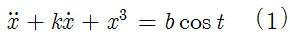
Since we can only use a single ODE, I will employ Ueda's oscillator model for illustration. The governing ODE is given by
 Here's the EquationTrekker code in Mathematica to generate the Poincaré section for Ueda's equations
Voila!
Once the equation trekker interface opens, you have to click on the little pencil icon at the top and then click inside the plane to specify the initial conditions. Of course, there's much more to say about equation trekker, but I leave that for your curiosity. To change the sampling interval (more or less points), just modify the integration range specified by t. The sampling frequency is specified by the "SectionCondition".
One can also easily generate the phase space using equation trekker. All you have to do is remove the TrekGenerator specification from the code given above, i.e.
Download Mathematica notebook [right click / save as]
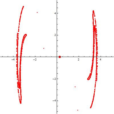
There is great package in Mathematica 6.x that enables us to solve differential equations with a snap. But that's not all, this package will automatically generate a user interface with real-time control of the parameters in the governing equations. This package is called EquationTrekker and is available in Mathematica 6.x. However, the only limitation of this package is that it works with a single first order or second order ODE. Also, EquationTrekker only displays phase diagrams and Poincaré sections. I have already discussed how one can generate the time series and the phase space diagram for a given dynamical system. In this article, I'll discuss how one can generate the Poincaré section using EquationTrekker.
Since we can only use a single ODE, I will employ Ueda's oscillator model for illustration. The governing ODE is given by
 Here's the EquationTrekker code in Mathematica to generate the Poincaré section for Ueda's equations
EquationTrekker[{x''[t] + k x'[t] + x[t]^3 == B Cos[t]}, x, {t, 0, 10000}, PlotRange -> {{-5, 5}, {-5, 5}}, TrekParameters -> {k -> 0.3, B -> 11.5}, TrekGenerator -> {PoincareSection, "SectionCondition" -> Mod[t, \[Pi]], "SectionVariables" -> {x, x'}, MaxSteps -> \[Infinity]}]

Voila!
Once the equation trekker interface opens, you have to click on the little pencil icon at the top and then click inside the plane to specify the initial conditions. Of course, there's much more to say about equation trekker, but I leave that for your curiosity. To change the sampling interval (more or less points), just modify the integration range specified by t. The sampling frequency is specified by the "SectionCondition".
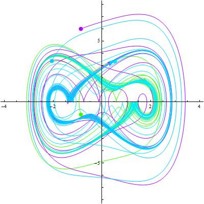
One can also easily generate the phase space using equation trekker. All you have to do is remove the TrekGenerator specification from the code given above, i.e.
EquationTrekker[{x''[t] + k x'[t] + x[t]^3 == B Cos[t]}, x, {t, 0, 100}, PlotRange -> {{-7, 7}, {-8, 8}}, TrekParameters -> {k -> 0.3, B -> 11.5}]

Download Mathematica notebook [right click / save as]
Cite as:
Saad, T. "Solving Differential Equations with Mathematica - Part IV: Equation Trekker".
Weblog entry from
Please Make A Note.
http://pleasemakeanote.blogspot.com/2008/05/solving-differential-equations-with_28.html
Sunday, May 25, 2008
Solving Differential Equations with Mathematica - Part III: Frequency Domain
Download Mathematica notebook [right click / save as]
Download Mathematica notebook [right click / save as]
In this article, we use a Fast Fourier Transform to study a dynamical system in the frequency domain. This conversion is very illuminating on the behavior of the dynamical system as it will point out the frequencies at which the system might become unstable or nonlinear. Using the results obtained in the first article of this series, Mathematica can easily convert the data into the frequency domain. This is accomplished by first generating a table containing the values obtained in the numerical solution and then applying a discrete Fourier transform to that data. The code that does this is given by
(* Generate a table containing the numerical solution *)Voila!
yvalues = Table[(x[t] /. s1)[[1]], {t, Tend}];
(* Apply a discrete Fourier transform on that data and plot it*)
ListLinePlot[Abs[Fourier[yvalues]], PlotRange -> All]
Download Mathematica notebook [right click / save as]
Cite as:
Saad, T. "Solving Differential Equations with Mathematica - Part III: Frequency Domain".
Weblog entry from
Please Make A Note.
http://pleasemakeanote.blogspot.com/2008/05/solving-differential-equations-with_25.html
Friday, May 23, 2008
Solving Differential Equations with Mathematica - Part II: Phase Space
Download Mathematica notebook [right click / save as]
To generate the 2D phase space, use this simple code
To generate the 3D phase space, use the ParametricPlot3D[] as follows
 Voila!
Download Mathematica notebook [right click / save as]
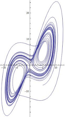
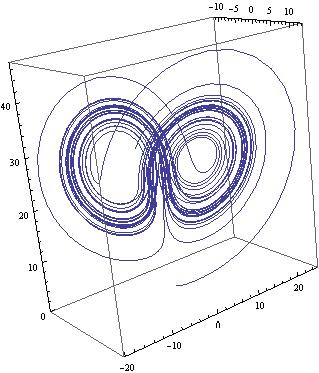
In a previous article, I discussed how one can use the NDSolve[] utility in Mathematica to obtain a numerical solution for a set of ODEs using the Lorenz equations as a representative example. In this article, I will show how easy it easy to plot the phase space diagram which represents all possible states for a given system. In the case of the Lorenz equations, the phase space is three dimensional because there are three variables: x, y, and z. But of course, one can always study subsets of the 3D phase space, i.e. x vs y for instance. To accomplish this, we make use of the numerical data generated in the previous article, and employ two function in Mathematica; ParametricPlot[] for 2D and ParametricPlot3D[] for 3D spaces.
To generate the 2D phase space, use this simple code
ParametricPlot[Evaluate[{x[t], y[t]} /. s1], {t, 0, Tend}, PlotRange -> All]

To generate the 3D phase space, use the ParametricPlot3D[] as follows
ParametricPlot3D[Evaluate[{x[t], y[t], z[t]} /. s1], {t, 0, Tend},PlotRange -> All]
 Voila!
Of course, s1 was obtained in Part I of this series and represents the numerical solution for the Lorenz equations.
Download Mathematica notebook [right click / save as]
Cite as:
Saad, T. "Solving Differential Equations with Mathematica - Part II: Phase Space".
Weblog entry from
Please Make A Note.
http://pleasemakeanote.blogspot.com/2008/05/solving-differential-equations-with_24.html
Thursday, May 22, 2008
Solving Differential Equations with Mathematica - Part I: Time Series
Download Mathematica notebook [right click / save as]
In this series, I will summarize some of the quickest methods to solve ordinary differential equations (ODEs hereafter) in Mathematica. To illustrate this, I will make use of the Lorenz dynamical system which is a set of three coupled ODEs. This dynamical system is notorious for its chaotic behavior and has given Lorenz the opportunity to be one of the first scientists who discovered chaos. In the process, I will also illustrate some of the techniques used to investigate chaotic behavior in dynamical systems; specifically, sensitivity to initial conditions, frequency domain transformations using the fast Fourier transform, and Poincaré sections.
The Lorenz equations are given by where x, y, and z are functions of time and sigma, rho, and beta are control parameters determined a priori. One could implement a fourth order Runga-Kutta method with adaptive time stepping to solve the above set of equations (and I would really recommend doing that). But in this article, we will use Mathematica which offers a super neat function called NDSolve[] that performs the numerical integration of ODEs. Without further adue, only a couple of lines of code are required in Mathematica to solve the above system of equations
Note that \[Sigma] will automatically convert to the greek symbol sigma. The same applies for the rest. You can also generate the greek letters by pressing escape, typing a letter on the keyboard, and then pressing escape. For example, escape, s, escape will turn into sigma.
Going back to the previous code, the two important statements are the NDSolve[] and the Plot[Evaluate[]].
In the first one, we are solving the Lorenz equations for x[t], y[t], and z[t] from t = 0 to t = Tend with an infinite number of time steps (MaxSteps->Infinity).
As for the Plot[Evaluate[]], the "x[t] /. s1" means replace all x[t] with the data contained in s1, which holds the results of the numerical integration. One could have also chosen to plot y[t] or z[t].
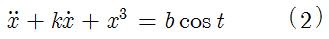
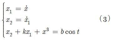
For first or higher order ODEs, it is advisable to get rid of all derivatives by definig them as new variables. This will be helpful for phase space diagrams to be discussed in the next article. For example, if you have the following system (Ueda's oscillator)
 it can be converted to
Download Mathematica notebook [right click / save as]
 where x, y, and z are functions of time and sigma, rho, and beta are control parameters determined a priori. One could implement a fourth order Runga-Kutta method with adaptive time stepping to solve the above set of equations (and I would really recommend doing that). But in this article, we will use Mathematica which offers a super neat function called NDSolve[] that performs the numerical integration of ODEs. Without further adue, only a couple of lines of code are required in Mathematica to solve the above system of equations
(* Define control parameters *)Voila!
\[Sigma] = 3; \[Beta] = 1; \[Rho] = 10;
(* Define initial conditions for later use *)
x0 = 0; y0 = 1; z0 = 1;
(* Define interval of integration *)
Tend = 20 \[Pi];
(* Lump the initial conditions in one variable *)
initialConditions = {x[0] == x0, y[0] == y0, z[0] == z0};
(* Lump the Lorenz equations in one variable *)
LorenzEquations = {x'[t] == \[Sigma] (y[t] - x[t]),
y'[t] == \[Rho] x[t] - x[t] z[t] - y[t],
z'[t] == x[t] y[t] - \[Beta] z[t],
initialConditions};
(* Use NDSolve to integrate the Lorenz equations *)
s1 = NDSolve[LorenzEquations, {x[t], y[t], z[t]}, {t, 0, Tend}, MaxSteps -> \[Infinity]];
(* Plot the solution *)
Plot[Evaluate[x[t] /. s1], {t, 0, Tend}, PlotRange -> All]
Note that \[Sigma] will automatically convert to the greek symbol sigma. The same applies for the rest. You can also generate the greek letters by pressing escape, typing a letter on the keyboard, and then pressing escape. For example, escape, s, escape will turn into sigma.
Going back to the previous code, the two important statements are the NDSolve[] and the Plot[Evaluate[]].
In the first one, we are solving the Lorenz equations for x[t], y[t], and z[t] from t = 0 to t = Tend with an infinite number of time steps (MaxSteps->Infinity).
As for the Plot[Evaluate[]], the "x[t] /. s1" means replace all x[t] with the data contained in s1, which holds the results of the numerical integration. One could have also chosen to plot y[t] or z[t].
For first or higher order ODEs, it is advisable to get rid of all derivatives by definig them as new variables. This will be helpful for phase space diagrams to be discussed in the next article. For example, if you have the following system (Ueda's oscillator)
 it can be converted to
Download Mathematica notebook [right click / save as]
Cite as:
Saad, T. "Solving Differential Equations with Mathematica - Part I: Time Series".
Weblog entry from
Please Make A Note.
http://pleasemakeanote.blogspot.com/2008/05/solving-differential-equations-with.html
Wednesday, May 21, 2008
Importing Vertex Data in Gambit
While still an undergraduate, one my CFD class projects was to analyze the flow over an airfoil. My first order of business was to figure out where I could obtain the airfoil profile (i.e. the coordinates of the vertices that define the airfoil profile). I eventually found the very useful NACA airfoil generator. It is a Java applet that runs in your (firefox) browser. It can be found here (4 digit series) or here (5 digit series).
Next, I had to figure out a way of input all the vertex data in Gambit. Obviously, it is very bad practice to input the data points one at a time. Being new to Gambit and CFD in general, my options were limited. Eventually, inputing the vertex data into Gambit turned out to be as easy as boiling eggs.
Next, I had to figure out a way of input all the vertex data in Gambit. Obviously, it is very bad practice to input the data points one at a time. Being new to Gambit and CFD in general, my options were limited. Eventually, inputing the vertex data into Gambit turned out to be as easy as boiling eggs.
Voila!
- Get the vertex data ready in a text file
- In Gambit, File->Import->Vertex Data
Note that if the data is two dimensional, the text file will have only two columns. Gambit, however, assumes this is 3D data and will mess things up. What you have to do in this case is add a third column to the data file and fill it with "0.0". You can do that manually, or write a code to do that for you. I've written a tiny application in C# that will append a value that you specify at the end of every line of a text file. You can download it from here.
Cite as:
Saad, T. "Importing Vertex Data in Gambit".
Weblog entry from
Please Make A Note.
http://pleasemakeanote.blogspot.com/2008/05/importing-vertex-data-in-gambit.html
Tuesday, May 20, 2008
Vector (Nabla) Operations in Curvilinear Coordinates
Vector calculus is an essential ingredient of modern scientific communication. First proposed by Josiah Willard Gibbs, vector analysis is compact, elegant, and simple. Fundamental components of vector analysis are the dot and cross product, as well as gradient, divergence, and curl. This post is intended as a quick and handy reminder of these various operations in different coordinates.
Dot and cross products are invariant under coordinate transformation, so they have the same form for all coordinates


Dot and cross products are invariant under coordinate transformation, so they have the same form for all coordinates
and
The remaining operations take specific forms under different coordinates. For Cylindrical coordinates

while for Spherical coordinates


Voila!
P.S. most people refer to the "inverted triangle" operator as the "del" operator; however, this symbol is called "nabla" just like epsilone, eta, gamma etc... and I find no reason for calling it otherwise! Therefore, I usually use terms such as "nabla phi" for the gradient of a scalar, "nabla dot A" and "nabla cross A" for the divergence and curl of a vector field, respectively.
P.S. most people refer to the "inverted triangle" operator as the "del" operator; however, this symbol is called "nabla" just like epsilone, eta, gamma etc... and I find no reason for calling it otherwise! Therefore, I usually use terms such as "nabla phi" for the gradient of a scalar, "nabla dot A" and "nabla cross A" for the divergence and curl of a vector field, respectively.
Cite as:
Saad, T. "Vector (Nabla) Operations in Curvilinear Coordinates".
Weblog entry from
Please Make A Note.
http://pleasemakeanote.blogspot.com/2008/05/nabla-operations-gradient-curl-and-dot.html
Convenient Form of the Navier-Stokes Equations
[NOTE: This post should have been updated a long time ago. I have cleaned it up to avoid any confusion. Thanks.]
Most of us learn the fundamentals of fluid mechanics using Cartesian coordinates. Specifically, derivations of the Navier-Stokes equations are done in a Cartesian reference system. This is a valid way for studying such a complicated set of equations as rectangular coordinates do not present us with the nuances of extra terms due to curvature or other effects that are present in curvilinear coordinates. The final form for the momentum equations is concisely written in vector notation for compactness and simplicity. This is given by
\mathbf{u}%20=%20\nu%20\nabla^2%20\mathbf{u}-\frac{1}{\rho}\nabla%20p%20+%20\mathbf{g} "\bg_white \120dpi \frac{\partial \mathbf{u}}{\partial t}+\left(\mathbf{u} \cdot \nabla \right )\mathbf{u} = \nu \nabla^2 \mathbf{u}-\frac{1}{\rho}\nabla p + \mathbf{g}")
\mathbf{u}%20=%20\nabla\left(\tfrac{1}{2}%20\mathbf{u}\cdot\mathbf{u}%20\right%20)-\mathbf{u}\times\nabla\times\mathbf{u} "\bg_white \120dpi \left(\mathbf{u} \cdot \nabla \right )\mathbf{u} = \nabla\left(\tfrac{1}{2} \mathbf{u}\cdot\mathbf{u} \right )-\mathbf{u}\times\nabla\times\mathbf{u}")
Most of us learn the fundamentals of fluid mechanics using Cartesian coordinates. Specifically, derivations of the Navier-Stokes equations are done in a Cartesian reference system. This is a valid way for studying such a complicated set of equations as rectangular coordinates do not present us with the nuances of extra terms due to curvature or other effects that are present in curvilinear coordinates. The final form for the momentum equations is concisely written in vector notation for compactness and simplicity. This is given by
Note that this is a vector equation yielding as many equations as there are coordinates.
In certain cases, it is important to express the convection term using the following identity
This form is very convenient for those of you working with analytical modeling of the NS equations. There was some confusion on whether this identity holds in general curvilinear coordinates. This identity is TRUE in general orthogonal curvilinear coordinates.
I would like to thank Prof. Gary Flandro of UTSI for promoting the use of this form.
I would like to thank Prof. Gary Flandro of UTSI for promoting the use of this form.
Cite as:
Saad, T. "Convenient Form of the Navier-Stokes Equations".
Weblog entry from
Please Make A Note.
http://pleasemakeanote.blogspot.com/2008/05/convenient-form-of-navier-stokes.html
Monday, May 19, 2008
Invariant Form of the Navier-Stokes Equations
This post has moved here
Cite as:
Saad, T. "Invariant Form of the Navier-Stokes Equations".
Weblog entry from
Please Make A Note.
http://pleasemakeanote.blogspot.com/2008/05/invariant-form-of-navier-stokes_20.html
Sunday, May 18, 2008
Interactive Plots in Mathematica
To study the behavior of an analytical solution that has several control parameters, one would usually plot that function under different combinations of these parameters. There is a super nice function in Mathematica that allows the user to dynamically plot the solution by changing the control parameters using sliders. The function is called Manipulate and here's an example
Manipulate[Plot[Exp[-w x] Cos[a x], {x, 0, 3 Pi}, PlotRange -> Full], {w, 0, 10}, {a, 0,20}]Voila!
The Manipulate[] function performs a job similar to that of the Table[] function, but with a graphical user interface. In the above code, we are manipulating a plot subject to two control parameters, w and a. The Plot[] function follows the standard Mathematica syntax. Here's a screen recording of how the result looks like
Of course, you can plot as many functions and accomodate as many control parameters as you want. This also works with 3D plots. Of course, you will have to use Plot3D to do that.
For a complete description of the Manipulate function, you can visit its Mathematica documentation page
http://reference.wolfram.com/mathematica/tutorial/IntroductionToManipulate.html
Cite as:
Saad, T. "Interactive Plots in Mathematica".
Weblog entry from
Please Make A Note.
http://pleasemakeanote.blogspot.com/2008/05/interactive-plots-in-mathematica.html
Saturday, May 17, 2008
Optimize Fluent Simulations
One way to optimize a Fluent simulation is to reorder the topology (i.e. cells, faces, and nodes) in memory so that accessing neighboring cell or face information induces a minimal overhead. According to Fluent, reordering the domain improves the performance of the solver. After reading the mesh file do the following
Grid->Reorder->DomainVoila!
You should notice some improvement in your simulation after performing the reordering operation. Make sure also to save the case file so that the reordering of the mesh is reflected in subsequent runs.
Cite as:
Saad, T. "Optimize Fluent Simulations".
Weblog entry from
Please Make A Note.
http://pleasemakeanote.blogspot.com/2008/05/optimize-fluent-simulations.html
Animations in Mathematica
Download Mathematica notebook [right click / save as]
A good way of presenting your work is to use animations. This is true when you have an analytical model where you need to explore the behavior of the solution under a change of certain control parameters. There's an easy way of doing this using Mathematica. Here is a sample code in mathematica

Voila!

Download Mathematica notebook [right click / save as]
A good way of presenting your work is to use animations. This is true when you have an analytical model where you need to explore the behavior of the solution under a change of certain control parameters. There's an easy way of doing this using Mathematica. Here is a sample code in mathematica
(* Define function to be animated *)The animation will look like this
f[x_, L_] = Cos[L*x];
(* Create a table of plots *)
theTable = Table[ Plot[{f[x, L]}, {x, -4, 4}], {L, 1, 10}];
(* Export this table into an animated GIF - Replace gif with swf to export as a flash swf file*)
Export["C:\\TestAnimation.gif", theTable, ImageSize->350];
Voila!
Of course, you need to set the parameters that are relevant to your animation. You can also animate several functions. In this case, include the functions in the Plot section of the table. For example
(* Define functions to be animated *)The animation in this case looks like this
f[x_, L_] = Cos[L*x];
g[x_, L_] = Sin[L*x];
(* Create a table of plots *)
theTable = Table[ Plot[{f[x, L], g[x, L]}, {x, -4, 4}], {L, 1, 10}];
(* Export this table into an animated GIF - Replace gif with swf to export as a flash swf file*)
Export["C:\\TestAnimationCombo.gif", theTable, ImageSize->350];

Download Mathematica notebook [right click / save as]
Cite as:
Saad, T. "Animations in Mathematica".
Weblog entry from
Please Make A Note.
http://pleasemakeanote.blogspot.com/2008/05/create-mathematica-swf-animation.html
Friday, May 16, 2008
Fluent Axisymmetric Simulations
To run an axisymmetric simulation in Fluent you have to do the following
- In Gambit, make sure your axis of symmetry is aligned with the x-axis (i.e. y = 0)
- Set the axis edge as an "axis" boundary condition
- Once you import your mesh into Fluent, set the solver to Axisymmetric
Voila!
Cite as:
Saad, T. "Fluent Axisymmetric Simulations".
Weblog entry from
Please Make A Note.
http://pleasemakeanote.blogspot.com/2008/05/fluent-axisymmetric-simulations.html
Thursday, May 15, 2008
Fluent Graphics Display in Remote Desktop Mode
Most of the time, I run my Fluent simulations on remote computers using the windows remote desktop. However, when trying to preview the solution, nothing appears in the graphics window. This is usually the case with 3D simulations. To fix this problem, you have to disable "Hidden Surface Removal" in the "Graphics Options" window
- Display->Options
- Uncheck "Hidden Surface Removal"
In 2D simulations, this option is usually unchecked. On the other hand, In 3D simulations, Fluent defaults to this option because it helps viewing 3D models.
Cite as:
Saad, T. "Fluent Graphics Display in Remote Desktop Mode".
Weblog entry from
Please Make A Note.
http://pleasemakeanote.blogspot.com/2008/05/fluent-graphics-display-in-remote.html
Wednesday, May 14, 2008
Set Column Values in Origin
Most of the times, when importing data into OriginLab, I need to normalize the data by a certain value, or perform certain calculations over each column. When this normalization or calculation is the same for all columns (i.e. normalize the column by 10) it is a hassle to go over each column, right click on it, select "Set Values", and then type in the formula for that column. This is tedious when my columns have long times. There a much easier way of doing this by using the "Before Formula Scripts". I know that this functionality is available as of Origin 8.0. Here's how I am currently doing it:
- Select the first column by clicking on its title label
- Right click and invoke the "Set Values" dialog box
- Click on the little arrow to the bottom right (called "Show Scripts")
- In the "Before Formula Scripts" text box, type in the following
// Get index of current column
const nn = _ThisColNum;
// Perform numerical operations on this column
wcol(nn) /= 10;
- Click apply
- Select the formula and copy it (Ctrl + c)
- Now go to the next column by clicking on the Next Column button (or simply selecting another column)
- Paste the formula (Ctrl + v) and click apply

I do this for all the columns. This process is very fast if you have a good handle on using the keyboard.
Cite as:
Saad, T. "Set Column Values in Origin".
Weblog entry from
Please Make A Note.
http://pleasemakeanote.blogspot.com/2008/05/set-column-values-in-origin.html
Tuesday, May 13, 2008
Enable LES (Large Eddy Simulation) in Fluent 2D
To enable Large Eddy Simulation for Fluent two dimensional models, open the Fluent main console and type the following:
This will enable LES in 2D models. Note that turbulence is inherently a 3D phenomenon and using LES for two dimensional flows is not recommended. However, in certain cases such as code benchmarks or debugging, it is useful to run LES in 2D. I would also speculate that LES is a valid model in axisymmetric conditions.
(rpsetvar 'les-2d? #t)Voila!
This will enable LES in 2D models. Note that turbulence is inherently a 3D phenomenon and using LES for two dimensional flows is not recommended. However, in certain cases such as code benchmarks or debugging, it is useful to run LES in 2D. I would also speculate that LES is a valid model in axisymmetric conditions.
Cite as:
Saad, T. "Enable LES (Large Eddy Simulation) in Fluent 2D".
Weblog entry from
Please Make A Note.
http://pleasemakeanote.blogspot.com/2008/05/enable-les-large-eddy-simulation-in.html
Monday, May 12, 2008
Automatically convert hyperlinks in MS Outlook 2008
When you are composing a new email in MS Outlook 2008, most of the time you will be inserting a hyperlink to a website. Depending on your email format settings, this "hyperlink" will not link anywhere, it will remain as regular text, such as this link
http://www.blogger.com/
Of course, it would be nicer if an internet address is automatically converted into a hyperlink, i.e.
http://www.blogger.com/
Outlook can do this automatically instead of manually converting each address into a clickable hyperlink. Here's how to do it:
http://www.blogger.com/
Of course, it would be nicer if an internet address is automatically converted into a hyperlink, i.e.
http://www.blogger.com/
Outlook can do this automatically instead of manually converting each address into a clickable hyperlink. Here's how to do it:
Voila!
- go to: Tools -> Options
- Click on the "Mail Format" tab
- Click on "Editor Options" at the bottom of the options dialog (this will bring up the "Editor Options" dialog)
- Click on the "Proofing" tab to your left
- Click on "AutoCorrect Options"
- Select "Internet and network paths with hyperlinks" in the "Replace as you type" section
Cite as:
Saad, T. "Automatically convert hyperlinks in MS Outlook 2008".
Weblog entry from
Please Make A Note.
http://pleasemakeanote.blogspot.com/2008/05/automatically-convert-hyperlinks-in-ms.html
Things to remember...
I created this blog for one obvious reason: I want to keep track of all the computer tricks I have used over the years to make my life and research easier. With new software popping up all over the place and with tons of new features, these sometimes hide the essential features that most of us look for and most often complicate the process of doing things in an efficient manner. As we grow older, it is difficult to keep track of all the nifty tricks that we knew when we were undergraduates. This blog is intended to help me remember all those goodies.
To make things easy (and in case you want to skip the reading as we all do when we are looking for a computer trick),
To make things easy (and in case you want to skip the reading as we all do when we are looking for a computer trick),
all the steps or codes required to achieve a certain task are typed in bule and placed in a dashed rectangleIn any event, I hope you find something useful on this blog. I would appreciate any comments.
Peace.
Cite as:
Saad, T. "Things to remember...".
Weblog entry from
Please Make A Note.
http://pleasemakeanote.blogspot.com/2008/05/things-to-remember.html
Subscribe to:
Comments (Atom)