Download Mathematica notebook [right click / save as]
In this series, I will summarize some of the quickest methods to solve ordinary differential equations (ODEs hereafter) in Mathematica. To illustrate this, I will make use of the Lorenz dynamical system which is a set of three coupled ODEs. This dynamical system is notorious for its chaotic behavior and has given Lorenz the opportunity to be one of the first scientists who discovered chaos. In the process, I will also illustrate some of the techniques used to investigate chaotic behavior in dynamical systems; specifically, sensitivity to initial conditions, frequency domain transformations using the fast Fourier transform, and Poincaré sections.
The Lorenz equations are given by where x, y, and z are functions of time and sigma, rho, and beta are control parameters determined a priori. One could implement a fourth order Runga-Kutta method with adaptive time stepping to solve the above set of equations (and I would really recommend doing that). But in this article, we will use Mathematica which offers a super neat function called NDSolve[] that performs the numerical integration of ODEs. Without further adue, only a couple of lines of code are required in Mathematica to solve the above system of equations
Note that \[Sigma] will automatically convert to the greek symbol sigma. The same applies for the rest. You can also generate the greek letters by pressing escape, typing a letter on the keyboard, and then pressing escape. For example, escape, s, escape will turn into sigma.
Going back to the previous code, the two important statements are the NDSolve[] and the Plot[Evaluate[]].
In the first one, we are solving the Lorenz equations for x[t], y[t], and z[t] from t = 0 to t = Tend with an infinite number of time steps (MaxSteps->Infinity).
As for the Plot[Evaluate[]], the "x[t] /. s1" means replace all x[t] with the data contained in s1, which holds the results of the numerical integration. One could have also chosen to plot y[t] or z[t].
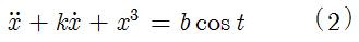
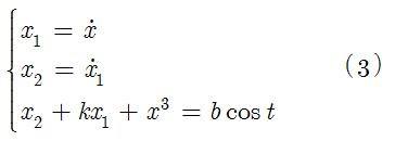
For first or higher order ODEs, it is advisable to get rid of all derivatives by definig them as new variables. This will be helpful for phase space diagrams to be discussed in the next article. For example, if you have the following system (Ueda's oscillator)
 it can be converted to
Download Mathematica notebook [right click / save as]
 where x, y, and z are functions of time and sigma, rho, and beta are control parameters determined a priori. One could implement a fourth order Runga-Kutta method with adaptive time stepping to solve the above set of equations (and I would really recommend doing that). But in this article, we will use Mathematica which offers a super neat function called NDSolve[] that performs the numerical integration of ODEs. Without further adue, only a couple of lines of code are required in Mathematica to solve the above system of equations
(* Define control parameters *)Voila!
\[Sigma] = 3; \[Beta] = 1; \[Rho] = 10;
(* Define initial conditions for later use *)
x0 = 0; y0 = 1; z0 = 1;
(* Define interval of integration *)
Tend = 20 \[Pi];
(* Lump the initial conditions in one variable *)
initialConditions = {x[0] == x0, y[0] == y0, z[0] == z0};
(* Lump the Lorenz equations in one variable *)
LorenzEquations = {x'[t] == \[Sigma] (y[t] - x[t]),
y'[t] == \[Rho] x[t] - x[t] z[t] - y[t],
z'[t] == x[t] y[t] - \[Beta] z[t],
initialConditions};
(* Use NDSolve to integrate the Lorenz equations *)
s1 = NDSolve[LorenzEquations, {x[t], y[t], z[t]}, {t, 0, Tend}, MaxSteps -> \[Infinity]];
(* Plot the solution *)
Plot[Evaluate[x[t] /. s1], {t, 0, Tend}, PlotRange -> All]
Note that \[Sigma] will automatically convert to the greek symbol sigma. The same applies for the rest. You can also generate the greek letters by pressing escape, typing a letter on the keyboard, and then pressing escape. For example, escape, s, escape will turn into sigma.
Going back to the previous code, the two important statements are the NDSolve[] and the Plot[Evaluate[]].
In the first one, we are solving the Lorenz equations for x[t], y[t], and z[t] from t = 0 to t = Tend with an infinite number of time steps (MaxSteps->Infinity).
As for the Plot[Evaluate[]], the "x[t] /. s1" means replace all x[t] with the data contained in s1, which holds the results of the numerical integration. One could have also chosen to plot y[t] or z[t].
For first or higher order ODEs, it is advisable to get rid of all derivatives by definig them as new variables. This will be helpful for phase space diagrams to be discussed in the next article. For example, if you have the following system (Ueda's oscillator)
 it can be converted to
Download Mathematica notebook [right click / save as]
Cite as:
Saad, T. "Solving Differential Equations with Mathematica - Part I: Time Series".
Weblog entry from
Please Make A Note.
http://pleasemakeanote.blogspot.com/2008/05/solving-differential-equations-with.html
very cool
ReplyDeleteThanks for the recommendation. I would like to start to use this program. the only downside it is that those programs usually don't show every step when there are solving a equation.
ReplyDeleteWhat a great post, I love mathematics, it is a fine and exact science.
ReplyDeleteCould you please reupload these files? There was removed and I would like to download them to learn how you do this calculations :) This series of posts, Part I-IV...doesn't work anymore :( Could somebody help me please?
ReplyDeleteI just updated all links to the Mathematica notebooks. Thanks for catching the broken links!
ReplyDeleteThank you very much! You are very kind!
ReplyDeleteI have one more question, if somebody could help me to solve one differential equation with mathematica? :(
In case there is somebody here who know well enough to use this program, my equation is:
(u`)^2+(5*mu*u-mu*u^3)u'-u^2=0
and I have to solve this equation around mu=-1;1;2;3 and to obtain some plots for each of these values:(.
I am stuck with this equation because I don't know how to use mathematica:(
Please help! :(
Thanks for providing helpful information...keep posting.......
ReplyDeletegeneric viagra
hi can you help me with this system of differential equation?
ReplyDeleteConsider the following predator-prey model: Let x1 denote the population
of adult prey, x2 the population of young prey and y the predator population.
Then
x˙1 = −a1x1 + a2x2 − bx1y
x˙2 = nx1 − (a1 + a2)x2
y˙ = −cy + dx1y
where all constants are nonnegative.
Find all equilibrium solutions of this system using mathematica.
thank you!
I would solve a system, which is almost the samen as the Lorenz system. I've made a few adjustments, but now the code doesn't work anymore... Can someone help me?
ReplyDeleteThis is my system:
u' = By - Cu
y' = uz - y
z' = - uy - (z-1)
with B=127 en C=3
This is Vallis sytem for El Niño. But I don't know the initial condition for this system. Maybe I can try some values?