Solving Differential Equations with Mathematica - Part II: Phase Space

Download Mathematica notebook [right click / save as]

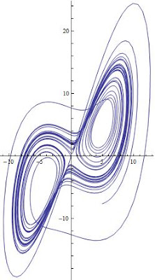
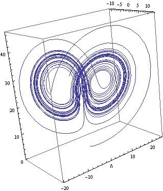
In a previous article, I discussed how one can use the NDSolve[] utility in Mathematica to obtain a numerical solution for a set of ODEs using the Lorenz equations as a representative example. In this article, I will show how easy it easy to plot the phase space diagram which represents all possible states for a given system. In the case of the Lorenz equations, the phase space is three dimensional because there are three variables: x, y, and z. But of course, one can always study subsets of the 3D phase space, i.e. x vs y for instance. To accomplish this, we make use of the numerical data generated in the previous article, and employ two function in Mathematica; ParametricPlot[] for 2D and ParametricPlot3D[] for 3D spaces.

To generate the 2D phase space, use this simple code

ParametricPlot[Evaluate[{x[t], y[t]} /. s1], {t, 0, Tend}, PlotRange -> All]

To generate the 3D phase space, use the ParametricPlot3D[] as follows

ParametricPlot3D[Evaluate[{x[t], y[t], z[t]} /. s1], {t, 0, Tend},PlotRange -> All]

Voila!

Of course, s1 was obtained in Part I of this series and represents the numerical solution for the Lorenz equations.

Download Mathematica notebook [right click / save as]

Cite as:
Saad, T. "Solving Differential Equations with Mathematica - Part II: Phase Space." Weblog entry from Please Make A Note. http://pleasemakeanote.blogspot.com/2008/05/solving-differential-equations-with_24.html