Download Mathematica notebook [right click / save as]
Since we can only use a single ODE, I will employ Ueda's oscillator model for illustration. The governing ODE is given by
 Here's the EquationTrekker code in Mathematica to generate the Poincaré section for Ueda's equations
Voila!
Once the equation trekker interface opens, you have to click on the little pencil icon at the top and then click inside the plane to specify the initial conditions. Of course, there's much more to say about equation trekker, but I leave that for your curiosity. To change the sampling interval (more or less points), just modify the integration range specified by t. The sampling frequency is specified by the "SectionCondition".
One can also easily generate the phase space using equation trekker. All you have to do is remove the TrekGenerator specification from the code given above, i.e.
Download Mathematica notebook [right click / save as]
There is great package in Mathematica 6.x that enables us to solve differential equations with a snap. But that's not all, this package will automatically generate a user interface with real-time control of the parameters in the governing equations. This package is called EquationTrekker and is available in Mathematica 6.x. However, the only limitation of this package is that it works with a single first order or second order ODE. Also, EquationTrekker only displays phase diagrams and Poincaré sections. I have already discussed how one can generate the time series and the phase space diagram for a given dynamical system. In this article, I'll discuss how one can generate the Poincaré section using EquationTrekker.
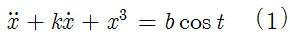
Since we can only use a single ODE, I will employ Ueda's oscillator model for illustration. The governing ODE is given by
 Here's the EquationTrekker code in Mathematica to generate the Poincaré section for Ueda's equations
EquationTrekker[{x''[t] + k x'[t] + x[t]^3 == B Cos[t]}, x, {t, 0, 10000}, PlotRange -> {{-5, 5}, {-5, 5}}, TrekParameters -> {k -> 0.3, B -> 11.5}, TrekGenerator -> {PoincareSection, "SectionCondition" -> Mod[t, \[Pi]], "SectionVariables" -> {x, x'}, MaxSteps -> \[Infinity]}]

Voila!
Once the equation trekker interface opens, you have to click on the little pencil icon at the top and then click inside the plane to specify the initial conditions. Of course, there's much more to say about equation trekker, but I leave that for your curiosity. To change the sampling interval (more or less points), just modify the integration range specified by t. The sampling frequency is specified by the "SectionCondition".
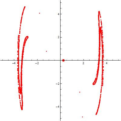
One can also easily generate the phase space using equation trekker. All you have to do is remove the TrekGenerator specification from the code given above, i.e.
EquationTrekker[{x''[t] + k x'[t] + x[t]^3 == B Cos[t]}, x, {t, 0, 100}, PlotRange -> {{-7, 7}, {-8, 8}}, TrekParameters -> {k -> 0.3, B -> 11.5}]

Download Mathematica notebook [right click / save as]
Cite as:
Saad, T. "Solving Differential Equations with Mathematica - Part IV: Equation Trekker".
Weblog entry from
Please Make A Note.
http://pleasemakeanote.blogspot.com/2008/05/solving-differential-equations-with_28.html
I am working on a project that models the double-pendulum system, undamped and undriven. I am having trouble setting up the Mathematica code in order to display the graphs of theta-dot vs. time, the phase-space portraits, and the poincare sections. As you may know, this system is a pair of coupled ordinary differential equations (second order), and I'm not sure if these can be plotted using EquationTrekker. If not, do you know of another way to accomplish the same task? Any input would be greatly appreciated as I am fairly unfamililar with Mathematica and am struggling to get these plots so that I can analyze them and complete my undergraduate thesis.
ReplyDeleteThank you for your comment.
ReplyDeleteAccording to the mathematica documentation, equation trekker can only handle a system of two first order ODEs.
Have you seen the Mathematica demonstration project on the double pendulum?
http://demonstrations.wolfram.com/DoublePendulum/
I hope this helps. Good luck with your work.
wow you solve that problem without use the viagra online theorem, you're a complete genius pal!
ReplyDeleteThis is really interesting because I didn't know I can get viagra online theorems, it should be something new in order to solve those equations, I'm really astonished with that.
ReplyDelete