Parallel Computing with MPI - Part VI: Parallel Computing in a Nutshell

Finally, we reach the most interesting part of this series. In this post, I will present, in a nutshell, the parts that you need to know in order to get started with parallel computing. I will base this discussion on an article that I wrote in 2005 on the CFD-Wiki. You can find it here. Of course, a lot has changed since then, but the basics and semantics are exactely the same. Any improvement that will happen in parallel computing will be at the implementation level, hardware, and additional functionality. The base has been laid out nicely and so it will remain for a while.

This article will be a very long one, albeit I hate to write long articles on a blog. So if you would like me to split it, just drop me a comment or an email.

What is Parallel Computing?

Parallel computing may be defined as the simultaneous use of several processors to execute a computer program. In the process, inter-processor communication is required at some point in the code; therefore, the code has to be instructed to run in parallel

For example, a code that computes the sum of the first N integers is very easy to program in parallel. Each processor will be responsible for computing a fraction of the global sum. However, at the end of the execution, all processors have to communicate their local sums to a single processor for example that will add them all up to obtain the global sum.

Types of Parallel Computers

There two types of parallel architectures

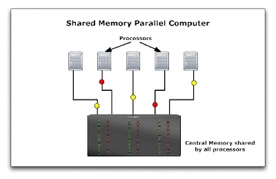
1. Shared memory multiprocessor
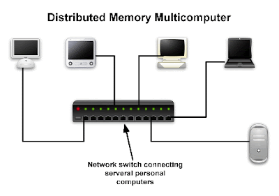
2. Distributed memory multicomputer

In a shared memory multiprocessor, all processors share the same "memory addresses". Imagine that these processors are all on the same motherboard. Multi-core CPUs (dual cores, quad cores) and multi CPU socket motherboards, such as server motherboards (or the computers we have in our offices at UTSI) are examples of a shared memory multiprocessor machine. In this setup, all processors have direct access to any of the variables declared in a code. This configuration is very attractive from a programming point of view: there is no need to send data from one computer to another. However, the main disadvantage lies in possible conflicts in accessing/altering data that resides in memory (imagine processor one is computing the temperature at a point, while processor two tries to access that same value for possible computation - in this case, there will be a conflict and memory cannot be accessed). This is usually remedied by inserting function calls to make that memory addresses can be accessed without conflict. Of course, this outweighs the benefits of sharing memory addresses and therefore this configuration is no longer popular since conflict management becomes a tedious and ambiguous process.


In a distributed memory configuration, each processor has its own memory addresses and data has to be sent from one processor to another. Computers are usually connected via network switch and data flows over the network from one processor to another. Note, however, that multi-core CPUs as well as multi-socket motherboards CAN use this configuration. In this case, although the memory modules are the same for all processors, each one of them reserves a portion of this memory just as if it existed independently of the others. Also, when multi-core systems are used, data is sent much faster since it does not have to go through a network. The main advantage of this configuration is robustness. For example, new machines can always be added to the parallel computer. Office computers can be used as part of the parallel computer when they are idle, and if the GRAs do not work overnight!



So How Does it Work?

The history of parallel computing extends over a long period of time and may be traced to the early 60's (check this link for a concise historical perspective). However, the most important milestone took place in 1992 when a bunch of scientist (most likely computer guys) were assembled to create a standard for message passing; their job was to formulate a universal framework for exchanging data in a parallel computer. So they retreated for a while and came up with what is called today the Message Passing Interface or MPI. It defines a set of functions and rules on how data is to flow from one processor to another within a parallel computer. Of course, they do not have to do the actual implementation as this is left for third party vendors or the open source community.

So how does parallel computing work? The notion is very simple. A computer code runs on different processors. At one point or another, data has to be exchanged between processors. Therefore, a functional call has to be included at that point to instruct the code to send or receive data. Once the executable reaches that line of code, it allocates some memory on the CPU buffer, copies the data that is to be sent, and sends this data to the receiving computer. On the receiving end, the code is waiting for some data to arrive. Of course, it knows what it will be receiving, therefore it allocates enough space in the CPU buffer and waits for this data. Once the data arrives, it copies it to the designated address in memory. and that's all!

Of course, there are many other ways that this happens, and different implementations do things differently, but the scenario presented above is one viable method. I still have to include some references though.

Cite as:
Saad, T. "Parallel Computing with MPI - Part VI: Parallel Computing in a Nutshell". Weblog entry from Please Make A Note. http://pleasemakeanote.blogspot.com/2008/06/parallel-computing-with-mpi-part-vi.html

Parallel Computing with MPI - Part V: MPICH2 and Visual Studio

Now that we have covered the sequential code for the finite difference solution of the 2D heat equation, It is time to start thinking in parallel. But first, we have to set the grounds for this adventure. This will be the topic of this post.

MPI, aka the Message Passing Interface, is a standard that defines a set of functions that allow a programmer to instruct their code to execute tasks in parallel. Of course, for this set of functions to be portable, they have to be compiled as a library. Then, the functions will be visible inside the code and used as necessary. I will defer my discussion on parallel computing to the next post as the sole purpose of this post is to have MPI ready so that we can experiment with it in our next post.

One thing that you have to understand is that MPI is a only a standard, but the implementations vary. This means that you will find several "MPI implementations" out there, some of them are free while others require the purchase of license, but nonetheless, they all offer the same functionality, function names, and datatypes as dictated by the MPI standard.

Fortunately, God created some people who are believe that science is not personal and are willing to take the time and put the effort to implement the MPI standard for free. The most popular implementations are the MPICH and the LamMPI. I use MPICH for windows and LamMPI for MacOSX.

For users of Unix based systems, I am going to assume that they have already enough knowledge on how to compile/install/link a library to their codes. Just do the same for MPI. You can download the MPICH2 implementation here and the LamMPI implementation here.

Now for windows users, I will outline the installation process of MPICH2 so that it is streamlined with Microsoft Visual Studio 2008. Both the express and professional editions can be used. Remember that the express edition can be downloaded for free!

I assume that you already have visual studio setup. There are two versions of MPICH2, namely, the 32 bit and 64 bit. For the time being, let us focus on the 32 bit version. Let us first setup the environment for MPI

1. Download and install MPICH2 32 bit edition
2. Add the following to your path
   C:\Program Files\MPICH2\bin
   (in Vista: right click My Computer/Properties/Advanced System Settings/Advanced/Environment Variables and edit the path variable for either the system or user variables - Do the same in XP, but you dont have to go through advanced system setting because it doesnt exist)
3. Add the following exceptions to your firewall:
   C:\Program Files\MPICH2\bin\mpiexec.exe
   C:\Program Files\MPICH2\bin\smpd.exe
   Usually, you will receive a message to unblock these programs. But in case you don't, you have to add them manually
   
4. Register a user account with MPI. Go to
   C:\Program Files\MPICH2\bin\wmpiregister
   and type in the user account and password that will be used to start MPI jobs. You should have the same user account and password on all your cluster machines
   
5. Open port 8676. Go to
   C:\Program Files\MPICH2\bin\wmpiconfig
   and select "port" at the top of the list

Note that if you install the 32 bit MPICH2 on a 64 bit windows, the MPICH installation directory will be under "Program Files (x86)".

Now, to setup the environment in Visual Studio we have to tell the compiler where to find the MPI header files and libraries, do the following

1. Start Visual Studio
2. Go to: Tools/Options/Projects and Solutions/Visual C++ Directories
3. In the platform combo box, select win32
4. In the Directories combo box, select "Include files" and add the following entry
   C:\Program Files\MPICH2\include (or Program Files (x86) for 64 bit windows)
5. Select "Library files" and add the following entry
   C:\Program Files\MPICH2\lib\ (or Program Files (x86) for 64 bit windows)

Voila!

Now your visual studio should be working like a charm! We'll test these settings in the next post.

Cite as:
Saad, T. "Parallel Computing with MPI - Part V: MPICH2 and Visual Studio". Weblog entry from Please Make A Note. http://pleasemakeanote.blogspot.com/2008/06/parallel-computing-with-mpi-part-v.html

Parallel Computing with MPI - Part IV: Programming the 2D Heat Equation in C using Visual Studio

Download c code | Download Visual Studio solution

In this post, you'll find the code that I have written for the numerical solution of the 2D heat equation. This is the sequential code, of course. By the way, sequential is the opposite of parallel, just in case you didn't know about it. There should be no confusion between sequential programming as all programming languages are sequential, i.e. the code is executed one line at a time.

To make things easy for newcomers, I have not used any extra header files to place the structure definitions as well as the function prototypes. Good programming practice, however, requries that you use header files to include function definitions, header files, and other stuff.

You will find two files over here. The first one, contains only the c code. Although the file extension is cpp, the code is in c. Using a C++ compiler will be perfect in this case.

The second is a rar archive and includes the visual studio solution files for those who wish to use visual studio C++ express. You can download it here. Simply extract the rar archive and open the ".sln" file.

The minimum that is expected from you is to read the whole code and understand before pressing the build or run buttons. I will most likely upload another version that has detailed comments on how things are done.

Download c code

Table of Contents:

1. Introducing the Heat Equation
2. Discretization of the Heat Equation
3. Stability Analysis and the Courant-Friedrichs-Lewy Criterion
4. Programming the Heat Equation in C using Visual Studio
5. MPICH2 and Visual Studio
6. Parallel Computing in a Nutshell
7. Measuring Parallel Performance
8. Essential Ingredients of Message Passing
   
9. MPI Warmup
   
10. Parallelizing the Heat Equation

Cite as:
Saad, T. "Parallel Computing with MPI - Part IV: Programming the 2D Heat Equation in C using Visual Studio". Weblog entry from Please Make A Note. http://pleasemakeanote.blogspot.com/2008/06/parallel-computing-with-mpi-part-iv.html

Parallel Computing with MPI - Part III: Stability Analysis of the Discretized Heat Equation

In today's part of this series, we'll go over a basic stability analysis for the discretized heat equation that was derived in the previous post.

Here, I will follow John Anderson's neat exposition of the stability analysis for difference equations. We start by defining a couple of terms first. Let,

D = exact solution of the difference equation (infinite accuracy computer)

N = numerical solution of the difference equation (finite accuracy computer)

ε = Round off error

then, by definition,

ε = N - D

which is the error between the exact solution and the finite accuracy numerical solution of the difference equation. Our difference equation can therefore be represented by N since we are most likely to solve it on a finite accuracy computer, right? To make headway, we replace T in our difference equation by N. at the outset, we get

(Eq. 1)

but, the numerical solution can be expressed in terms of the round off error and the exact difference equation solution as

(Eq. 2)

If we substitute this into the difference equation, we get

(Eq. 3)

however, the exact solution D to the difference equation already satisfies the discretized equation. Then, D simply cancels out from the above equation, and therefore, the round off error also satisfies the difference equation, i.e.

(Eq. 4)

Since we are solving using a real computer, then round off errors are inevitable. Therefore, we want to study how these errors evolve from one timestep to another. If ε gets smaller or at worst stays the same, then the solution is stable. Otherwise, it gets larger, then the solution is unstable. Mathematically, for a numerical solution to be stable, this can be expressed as

(Eq. 5)

Now, we wish to seek a general form of the round off error. Thankfully, once upon a time, a mathematician called Joseph Fourier showed that any function can be expressed as an infinite series of sines and cosines, or more conveniently, exponentials. Therefore, it is reasonable to assume the following general form for the round off error

(Eq. 6)

where i is the imaginary unit, kn is a wave number, and An(t) reflects the time dependence of the round off error. One may also assume a general form for An(t). Since the error will either grow or decay with time, then one can set

(Eq. 7)

so that the general form of the round off error is

(Eq. 8)

Now, we can substitute this form into the discretized equation accordingly. For example,

(Eq. 9)

Upon substitution and simplification, i.e. dividing by ε(x,y,t), we get

(Eq. 10)

nice! Notice that the infinite sum is no longer needed. Also, the exponential terms inside the parentheses can be collapsed into cosines

(Eq. 11)

This form, albeit quite simple, does not help in the subsequent steps. We need to invoke one extra trigonometric identity

(Eq. 12)

to obtain

(Eq. 13)

Now we take the absolute value of this equation and obtain the stability requirement

(Eq. 14)

we get two cases

Case I:

(Eq. 15)

or

(Eq. 16)

which is always true. So this case does not pose any limitations.

Case II:

(Eq. 17)

or

(Eq. 18)

but, since the square of the sine is always less than or equal to 1, then

(Eq. 19)

going back to the original inequality, for stability, we must satisfy

(Eq. 20)

or

(Eq. 21)

This is known as the Courant-Friedrichs-Lewy or the CFL condition. Although not in the context in which it was originally derived, a CFL condition may be obtained for almost any numerical analysis of differential equation.

In general, if the grid spacing was not uniform, we would have

(Eq. 22)

Note that in Horak and Gruber's paper (Parallel Numerical Solution of 2-D Heat Equation), there is a typo in the stability condition equation on page 49 (first equation on that page). The "2" in the denominator should actually be a "4" as was shown in this post. The CFL condition that the authors refer to actually corresponds to the one dimensional heat equation.

In my next post, I'll post a sequential program for solving the heat equation in C using visual studio.

REFERENCES

1. ANDERSON, J. D. 1995 Computational fluid dynamics : the basics with applications. McGraw-Hill.

2. TANNEHILL, J. C., ANDERSON, D. A. & PLETCHER, R. H. 1997 Computational fluid mechanics and heat transfer. 2nd edn. Taylor & Francis.

Table of Contents:

1. Introducing the Heat Equation
2. Discretization of the Heat Equation
3. Stability Analysis and the Courant-Friedrichs-Lewy Criterion
4. Programming the Heat Equation in C using Visual Studio
5. MPICH2 and Visual Studio
6. Parallel Computing in a Nutshell
7. Measuring Parallel Performance
8. Essential Ingredients of Message Passing
   
9. MPI Warmup
   
10. Parallelizing the Heat Equation

Cite as:
Saad, T. "Parallel Computing with MPI - Part III: Stability Analysis of the Discretized Heat Equation". Weblog entry from Please Make A Note. http://pleasemakeanote.blogspot.com/2008/06/parallel-computing-with-mpi-part-iii.html

Parallel Computing with MPI - Part II: Discretization of the Heat Equation

In this article, we'll discuss how to discretize the heat equation using an Euler explicit differencing schem. The discretization is first order forward in time, and second order central in space. I am assuming that you are somehow familiar with finite difference methods. If not, then discuss it with your therapist.

Again, we are considering the heat equation given by

The underlying idea in discretization is to first divide the domain of interest (i.e. the region over which we are solving the heat equation) into a grid of discrete points (in space and time). When this is done, the derivatives can be approximated using the values of the dependent variable T at the discrete points. For convenience, the grid points are indexed using i in the horizontal x direction, and j in the vertical y direction.

Similarly, the time dimension is divided into time levels n, n+1, n+2... separated by a timestep Δt.

Next, we have to transform Eq. (1) into an algebraic relation at (any) point (i, j) and time level n. To do this, we have to convert each derivative into an equivalent algebraic expression. For the unsteady term, we use a forward Euler scheme as follows


where n denotes the time level and Δt denotes the timestep size. The form given in Eq. (2) is called forward in time because it uses the value of T at the next time level (n+1), which is unknown. In essence, we are solving for T at (n+1)

For the spatial derivatives, we will use explicit central differencing. This means that the discretized form of the spatial derivatives will be evaluated at the current time level n where the values are known. This is written as

and
If we further allow Δx = Δy = δ Upon substitution of Eqs. (2)-(4) into Eq. (1), we obtain the full discretized form of the heat equation


finally, the simplicity of the explicit scheme is clearly visible in Eq. (5) as one can easily solve for the new time level (n+1)
This means that there is no need to solve a linear system of equations. If we had used an implicit method, the RHS of Eq. (6) would be at time level (n + 1) and therefore, one would have to solve a linear system of equations at each time step.

In the next post, we'll discuss the stability of the discretized equation and derive the CFL criterion to ensure stability of the numerical solution given by Eq. (6).

Table of Contents:

1. Introducing the Heat Equation
2. Discretization of the Heat Equation
3. Stability Analysis and the Courant-Friedrichs-Lewy Criterion
4. Programming the Heat Equation in C using Visual Studio
5. MPICH2 and Visual Studio
6. Parallel Computing in a Nutshell
7. Measuring Parallel Performance
8. Essential Ingredients of Message Passing
   
9. MPI Warmup
   
10. Parallelizing the Heat Equation

Cite as:
Saad, T. "Parallel Computing with MPI - Part II: Discretization of the Heat Equation". Weblog entry from Please Make A Note. http://pleasemakeanote.blogspot.com/2008/06/parallel-computing-with-mpi-part-ii.html