Cite as:
Saad, T. "Solving Differential Equations with Mathematica - Roundup".
Weblog entry from
Please Make A Note.
http://pleasemakeanote.blogspot.com/2008/05/solving-differential-equations-with_29.html?m=0
Wednesday, May 28, 2008
Solving Differential Equations with Mathematica - Roundup
This is a roundup of the posts for solving differential equations with Mathematica. This was illustrated using the Lorentz equations. The topics that were discussed are as follows:

Solving Differential Equations with Mathematica - Part IV: Equation Trekker
Download Mathematica notebook [right click / save as]
Since we can only use a single ODE, I will employ Ueda's oscillator model for illustration. The governing ODE is given by
 Here's the EquationTrekker code in Mathematica to generate the Poincaré section for Ueda's equations
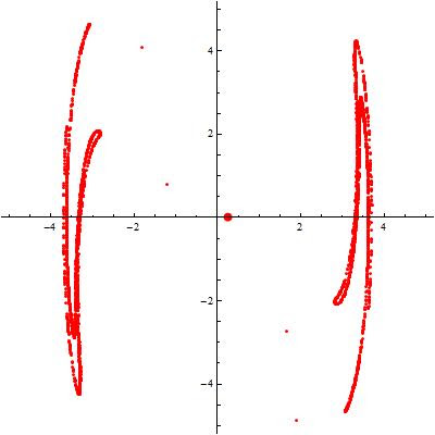
Voila!
Once the equation trekker interface opens, you have to click on the little pencil icon at the top and then click inside the plane to specify the initial conditions. Of course, there's much more to say about equation trekker, but I leave that for your curiosity. To change the sampling interval (more or less points), just modify the integration range specified by t. The sampling frequency is specified by the "SectionCondition".
One can also easily generate the phase space using equation trekker. All you have to do is remove the TrekGenerator specification from the code given above, i.e.
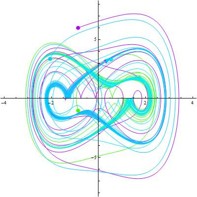
Download Mathematica notebook [right click / save as]
There is great package in Mathematica 6.x that enables us to solve differential equations with a snap. But that's not all, this package will automatically generate a user interface with real-time control of the parameters in the governing equations. This package is called EquationTrekker and is available in Mathematica 6.x. However, the only limitation of this package is that it works with a single first order or second order ODE. Also, EquationTrekker only displays phase diagrams and Poincaré sections. I have already discussed how one can generate the time series and the phase space diagram for a given dynamical system. In this article, I'll discuss how one can generate the Poincaré section using EquationTrekker.
Since we can only use a single ODE, I will employ Ueda's oscillator model for illustration. The governing ODE is given by
 Here's the EquationTrekker code in Mathematica to generate the Poincaré section for Ueda's equations
EquationTrekker[{x''[t] + k x'[t] + x[t]^3 == B Cos[t]}, x, {t, 0, 10000}, PlotRange -> {{-5, 5}, {-5, 5}}, TrekParameters -> {k -> 0.3, B -> 11.5}, TrekGenerator -> {PoincareSection, "SectionCondition" -> Mod[t, \[Pi]], "SectionVariables" -> {x, x'}, MaxSteps -> \[Infinity]}]

Voila!
Once the equation trekker interface opens, you have to click on the little pencil icon at the top and then click inside the plane to specify the initial conditions. Of course, there's much more to say about equation trekker, but I leave that for your curiosity. To change the sampling interval (more or less points), just modify the integration range specified by t. The sampling frequency is specified by the "SectionCondition".
One can also easily generate the phase space using equation trekker. All you have to do is remove the TrekGenerator specification from the code given above, i.e.
EquationTrekker[{x''[t] + k x'[t] + x[t]^3 == B Cos[t]}, x, {t, 0, 100}, PlotRange -> {{-7, 7}, {-8, 8}}, TrekParameters -> {k -> 0.3, B -> 11.5}]

Download Mathematica notebook [right click / save as]
Cite as:
Saad, T. "Solving Differential Equations with Mathematica - Part IV: Equation Trekker".
Weblog entry from
Please Make A Note.
http://pleasemakeanote.blogspot.com/2008/05/solving-differential-equations-with_28.html?m=0
Sunday, May 25, 2008
Solving Differential Equations with Mathematica - Part III: Frequency Domain
Download Mathematica notebook [right click / save as]
Download Mathematica notebook [right click / save as]
In this article, we use a Fast Fourier Transform to study a dynamical system in the frequency domain. This conversion is very illuminating on the behavior of the dynamical system as it will point out the frequencies at which the system might become unstable or nonlinear. Using the results obtained in the first article of this series, Mathematica can easily convert the data into the frequency domain. This is accomplished by first generating a table containing the values obtained in the numerical solution and then applying a discrete Fourier transform to that data. The code that does this is given by
(* Generate a table containing the numerical solution *)Voila!
yvalues = Table[(x[t] /. s1)[[1]], {t, Tend}];
(* Apply a discrete Fourier transform on that data and plot it*)
ListLinePlot[Abs[Fourier[yvalues]], PlotRange -> All]
Download Mathematica notebook [right click / save as]
Cite as:
Saad, T. "Solving Differential Equations with Mathematica - Part III: Frequency Domain".
Weblog entry from
Please Make A Note.
http://pleasemakeanote.blogspot.com/2008/05/solving-differential-equations-with_25.html?m=0
Friday, May 23, 2008
Solving Differential Equations with Mathematica - Part II: Phase Space
Download Mathematica notebook [right click / save as]
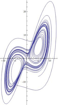
To generate the 2D phase space, use this simple code
To generate the 3D phase space, use the ParametricPlot3D[] as follows
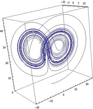 Voila!
Download Mathematica notebook [right click / save as]
In a previous article, I discussed how one can use the NDSolve[] utility in Mathematica to obtain a numerical solution for a set of ODEs using the Lorenz equations as a representative example. In this article, I will show how easy it easy to plot the phase space diagram which represents all possible states for a given system. In the case of the Lorenz equations, the phase space is three dimensional because there are three variables: x, y, and z. But of course, one can always study subsets of the 3D phase space, i.e. x vs y for instance. To accomplish this, we make use of the numerical data generated in the previous article, and employ two function in Mathematica; ParametricPlot[] for 2D and ParametricPlot3D[] for 3D spaces.
To generate the 2D phase space, use this simple code
ParametricPlot[Evaluate[{x[t], y[t]} /. s1], {t, 0, Tend}, PlotRange -> All]

To generate the 3D phase space, use the ParametricPlot3D[] as follows
ParametricPlot3D[Evaluate[{x[t], y[t], z[t]} /. s1], {t, 0, Tend},PlotRange -> All]
 Voila!
Of course, s1 was obtained in Part I of this series and represents the numerical solution for the Lorenz equations.
Download Mathematica notebook [right click / save as]
Cite as:
Saad, T. "Solving Differential Equations with Mathematica - Part II: Phase Space".
Weblog entry from
Please Make A Note.
http://pleasemakeanote.blogspot.com/2008/05/solving-differential-equations-with_24.html?m=0
Thursday, May 22, 2008
Solving Differential Equations with Mathematica - Part I: Time Series
Download Mathematica notebook [right click / save as]
In this series, I will summarize some of the quickest methods to solve ordinary differential equations (ODEs hereafter) in Mathematica. To illustrate this, I will make use of the Lorenz dynamical system which is a set of three coupled ODEs. This dynamical system is notorious for its chaotic behavior and has given Lorenz the opportunity to be one of the first scientists who discovered chaos. In the process, I will also illustrate some of the techniques used to investigate chaotic behavior in dynamical systems; specifically, sensitivity to initial conditions, frequency domain transformations using the fast Fourier transform, and Poincaré sections.
The Lorenz equations are given by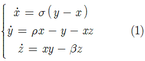 where x, y, and z are functions of time and sigma, rho, and beta are control parameters determined a priori. One could implement a fourth order Runga-Kutta method with adaptive time stepping to solve the above set of equations (and I would really recommend doing that). But in this article, we will use Mathematica which offers a super neat function called NDSolve[] that performs the numerical integration of ODEs. Without further adue, only a couple of lines of code are required in Mathematica to solve the above system of equations
Note that \[Sigma] will automatically convert to the greek symbol sigma. The same applies for the rest. You can also generate the greek letters by pressing escape, typing a letter on the keyboard, and then pressing escape. For example, escape, s, escape will turn into sigma.
Going back to the previous code, the two important statements are the NDSolve[] and the Plot[Evaluate[]].
In the first one, we are solving the Lorenz equations for x[t], y[t], and z[t] from t = 0 to t = Tend with an infinite number of time steps (MaxSteps->Infinity).
As for the Plot[Evaluate[]], the "x[t] /. s1" means replace all x[t] with the data contained in s1, which holds the results of the numerical integration. One could have also chosen to plot y[t] or z[t].
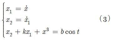
For first or higher order ODEs, it is advisable to get rid of all derivatives by definig them as new variables. This will be helpful for phase space diagrams to be discussed in the next article. For example, if you have the following system (Ueda's oscillator)
 it can be converted to
Download Mathematica notebook [right click / save as]
 where x, y, and z are functions of time and sigma, rho, and beta are control parameters determined a priori. One could implement a fourth order Runga-Kutta method with adaptive time stepping to solve the above set of equations (and I would really recommend doing that). But in this article, we will use Mathematica which offers a super neat function called NDSolve[] that performs the numerical integration of ODEs. Without further adue, only a couple of lines of code are required in Mathematica to solve the above system of equations
(* Define control parameters *)Voila!
\[Sigma] = 3; \[Beta] = 1; \[Rho] = 10;
(* Define initial conditions for later use *)
x0 = 0; y0 = 1; z0 = 1;
(* Define interval of integration *)
Tend = 20 \[Pi];
(* Lump the initial conditions in one variable *)
initialConditions = {x[0] == x0, y[0] == y0, z[0] == z0};
(* Lump the Lorenz equations in one variable *)
LorenzEquations = {x'[t] == \[Sigma] (y[t] - x[t]),
y'[t] == \[Rho] x[t] - x[t] z[t] - y[t],
z'[t] == x[t] y[t] - \[Beta] z[t],
initialConditions};
(* Use NDSolve to integrate the Lorenz equations *)
s1 = NDSolve[LorenzEquations, {x[t], y[t], z[t]}, {t, 0, Tend}, MaxSteps -> \[Infinity]];
(* Plot the solution *)
Plot[Evaluate[x[t] /. s1], {t, 0, Tend}, PlotRange -> All]
Note that \[Sigma] will automatically convert to the greek symbol sigma. The same applies for the rest. You can also generate the greek letters by pressing escape, typing a letter on the keyboard, and then pressing escape. For example, escape, s, escape will turn into sigma.
Going back to the previous code, the two important statements are the NDSolve[] and the Plot[Evaluate[]].
In the first one, we are solving the Lorenz equations for x[t], y[t], and z[t] from t = 0 to t = Tend with an infinite number of time steps (MaxSteps->Infinity).
As for the Plot[Evaluate[]], the "x[t] /. s1" means replace all x[t] with the data contained in s1, which holds the results of the numerical integration. One could have also chosen to plot y[t] or z[t].
For first or higher order ODEs, it is advisable to get rid of all derivatives by definig them as new variables. This will be helpful for phase space diagrams to be discussed in the next article. For example, if you have the following system (Ueda's oscillator)
 it can be converted to
Download Mathematica notebook [right click / save as]
Cite as:
Saad, T. "Solving Differential Equations with Mathematica - Part I: Time Series".
Weblog entry from
Please Make A Note.
http://pleasemakeanote.blogspot.com/2008/05/solving-differential-equations-with.html?m=0
Subscribe to:
Posts (Atom)